Peak Picking in 4D Spectrum with POKY

Overview

The general workflow of this tutorial starts with referencing and converting the spectra to POKY/Sparky format. Then, we will create 2D projections from the 4D spectrum, which will help us reference it properly.

For peak picking, we will follow a systematic strategy that, although more involved, will allow for higher precision in identifying peaks in the 4D spectrum while minimizing noise. Since the 2D projections are derived directly from the 4D spectrum, they provide a more accurate reference than the HSQC spectra, whose peak centers may deviate slightly from those in the projections.

To ensure accurate peak selection, we will use the 2D projections as intermediate reference points for restricted peak picking in the 4D spectrum. The workflow is as follows:

1. Overlay the projections onto the corresponding HSQC spectra
2. Identify peak centers by using the HSQC spectra as references
3. Use these peak centers to perform restricted peak picking in the 4D spectrum
4. Unfold or unalias peaks as necessary
5. Remove noise peaks from the 4D spectrum

By following this approach, we ensure that the final set of picked peaks in the 4D spectrum is as accurate and noise-free as possible.

Prerequisites

• Installation of POKY or NMRFAM-Sparky; license for POKY.
• Copy the enhanced Restricted Peak Pick POKY plugin that reads the tolerance values from the peak’s “Note” field from nmr_tutorials/SPARKY_and_POKY/POKY/scripts/restrictedpick.py to your POKY/poky_linux/modules/poky/ folder.
• Access to the specified CA2 protein 4D HCNH NOESY, 15N HSQC and 13C HSQC spectrum files.

Steps

---

Step 1. Reference the HSQC Spectra in Topspin

Follow the instructions to reference the 1H-15N and 1H-13C HSQC in Topspin with BioTop.

---

Step 2. Convert and Prepare Spectra

2.1 Convert Spectra to UCSF Format

Enter the directory where each spectrum is saved in Bruker format and run bruk2ucsf from there—running it from another directory will fail.
For example, to convert the 1H-15N, 1H-13C HSQC spectra, and the 4D HCNH NOESY:

 bruk2ucsf_run 6/pdata/1/2rr /srv/NMR/Peak_Picking/Nanoluc/15N_HSQC.ucsf
 bruk2ucsf_run 7/pdata/1/2rr /srv/NMR/Peak_Picking/Nanoluc/13C_HSQC.ucsf
 bruk2ucsf_run 5/pdata/1/4rrr /srv/NMR/Peak_Picking/Nanoluc/4D_HCNH_NOESY.ucsf

Note: You can also convert the spectra from Bruker to UCSF format in POKY/Sparky, but you cannot rename the axes in that process.

2.2 Rename Axes

Rename the axes in the 1H-15N and 1H-13C HSQC spectra:

ucsfdata -a1 N -a2 HN 15N_HSQC.ucsf
ucsfdata -a1 C -a2 HC 13C_HSQC.ucsf

Print the axis values of the 4D HCNH NOESY:

ucsfdata 4D_HCNH_NOESY.ucsf

Example output:

axis                          w1          w2          w3          w4
nucleus                       1H         13C         15N          1H
matrix size                  256         256         256         416
block size                     8           8           8          13
upfield ppm                1.194       6.301     101.402       5.279
downfield ppm              8.208      73.001     133.002      10.622
spectrum width Hz       6666.667   15939.978    3043.445    5078.125
transmitter MHz          950.374     238.980      96.311     950.374

From the upfield and downfield rows, you can guess which axis is HC and which is HN. In this example, the following command renames them properly—amide protons have higher shift values than the aliphatic protons:

ucsfdata -a1 HC -a2 C -a3 N -a4 HN 4D_HCNH_NOESY.ucsf

IMPORTANT: Make sure that axes are named consistently in all spectra; otherwise, you will encounter problems during peak picking.

2.3 Create C-HC and N-HN Projections

For a detailed tutorial, see Create_2D_projections_from_4D_spectrum. Briefly, extract the N-HN projection from the 4D HCNH NOESY. You may need to adjust the -p[1-4] values according to your 4D spectrum dimension order:

ucsfdata -p1 -r -o C-N-HN.ucsf 4D_HCNH_NOESY.ucsf
ucsfdata -p1 -r -o 2D_N-HN_proj.ucsf C-N-HN.ucsf

Similarly, for the C-HC projection:

ucsfdata -p4 -r -o HC-C-N.ucsf 4D_HCNH_NOESY.ucsf
ucsfdata -p3 -r -o 2D_HC-C_proj.ucsf HC-C-N.ucsf

---

Step 3. Loading the Spectra

Load the spectra

• Open the UCSF files with the fo command (make sure to display Poky Spectrum type of files in the pop-up browser), navigate to the folder, and select your spectra. Alternatively, you can copy the full path to each spectrum (for example, realpath 4D_HCNH_NOESY.ucsf in the Shell) and paste it into the pop-up browser.
• Do the same with the 2D projections and the HSQC spectra.
• Use xa to show the nucleus types on the axes; xr to roll the axes and xx to transpose them.
• Fix the aspect ratio by hitting vt and increasing the Aspect (ppm), for example, to 12, and then Apply.

---

Step 4. Adjusting the Spectra

Synchronize Spectra

• Click yt to synchronize the N axes of the 1H-15N HSQC and 4D_HCNH_NOESY first, and then synchronize the HN axes of those same spectra. Remember to synchronize one axis at a time!
• Do the same for the 1H-13C HSQC and 4D_HCNH_NOESY, and then for both HSQC spectra and the respective 2D projections.

Correct the contour levels and colors

• Type vC to bring up the contour level control scrollbars and adjust the contour levels.
• Type ec to bring up the easy contour dialog allowing you to adjust all loaded spectra, including their colors.
• If you double-click on a spectrum in the dialog it will open up the contour level dialog (equivalent to the ct command).

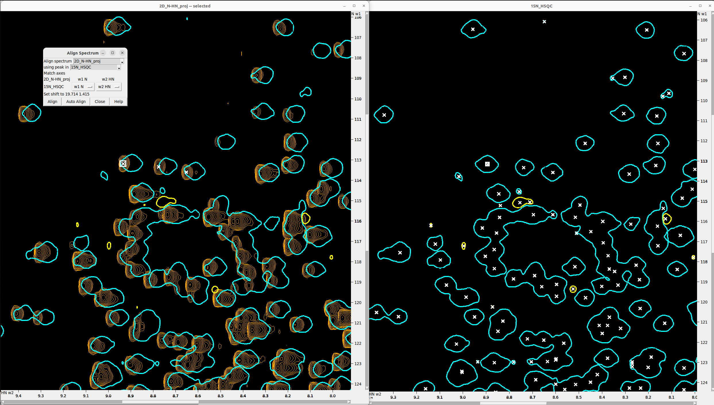
Align the 2D_N-HN_proj to the 15N_HSQC

• The 4D axes are usually completely off and must be aligned to the reference HSQC spectra. To achieve this, use the 2D projections.
• Hit ol to overlay 2D_N-HN_proj.ucsf onto 15N_HSQC.
• You may reduce the contour number to 1 for one of the two spectra for better visibility. Also hit oz to increase the contour thickness and the peak marker thickness.
• Manually pick the most “trustworthy” peak in the 15N_HSQC (F8 to enter peak picking mode, F1 to exit it) and find the same peak in the 4D.
• Type al, and in the pop-up:
  • Set Align spectrum to 2D_N-HN_proj
  • Set using peak in to 15N_HSQC
  • The axes should match, thanks to the renaming we did earlier.
  • Now hold the Shift key and select one “trustworthy” peak in each spectrum for alignment.
  • Hit Align.
  • Alternatively pick a set of matching peaks (button F8) in both spectra and click the Auto align option (slower and does not always work well).

Align the 2D_HC-C_proj to the 13C_HSQC
Follow the same procedure described in the previous step.

Reference the 4D_HCNH_NOESY

• Hit st and copy the shift values from the aligned 2D_N-HN_proj to 4D_HCNH_NOESY.
• Make sure that every time you copy a shift value from one spectrum to the other, you click Apply, or else the value is not saved.
• Similarly, copy the shift values from the aligned 2D_HC-C_proj to 4D_HCNH_NOESY.
• When you finish, click OK, and the 4D_HCNH_NOESY will be referenced!

---

Step 5. Peak Picking

5.1 Adjusting Contour Levels and Preparing Reference Peaks

• Adjust the contour levels (both positive and negative) in the 15N HSQC spectrum to optimize peak visibility.
• Press F8 to enter peak picking mode and select all visible peaks.
• Use the following Python function to estimate the expected number of N-H (in-phase) peaks from the amino acid sequence in the 15N HSQC:

  def estimate_15N_hsqc_peaks(sequence: str) -> int:
    # Count backbone amides = total residues minus any prolines and the N-terminus
    backbone_peaks = sum(1 for aa in sequence if aa != 'P') -1
    # Count side-chain peaks from R (NE–HE), K (NZ–QZ), W (NE1–HE1), and H (ND1-HD1)
    sidechain_peaks = sequence.count('R') + sequence.count('K') + sequence.count('W') + sequence.count('H')
    return backbone_peaks + sidechain_peaks
  

• Gradually increase or decrease the contour levels until the number of in-phase (positive intensity) picked peaks is approximately the expected number of N-H peaks (292 for CA2 protein). I set the contour level to 1.4e+06, which captured 274 in-phase peaks, as below that a lot of noise peaks were emerging.

  

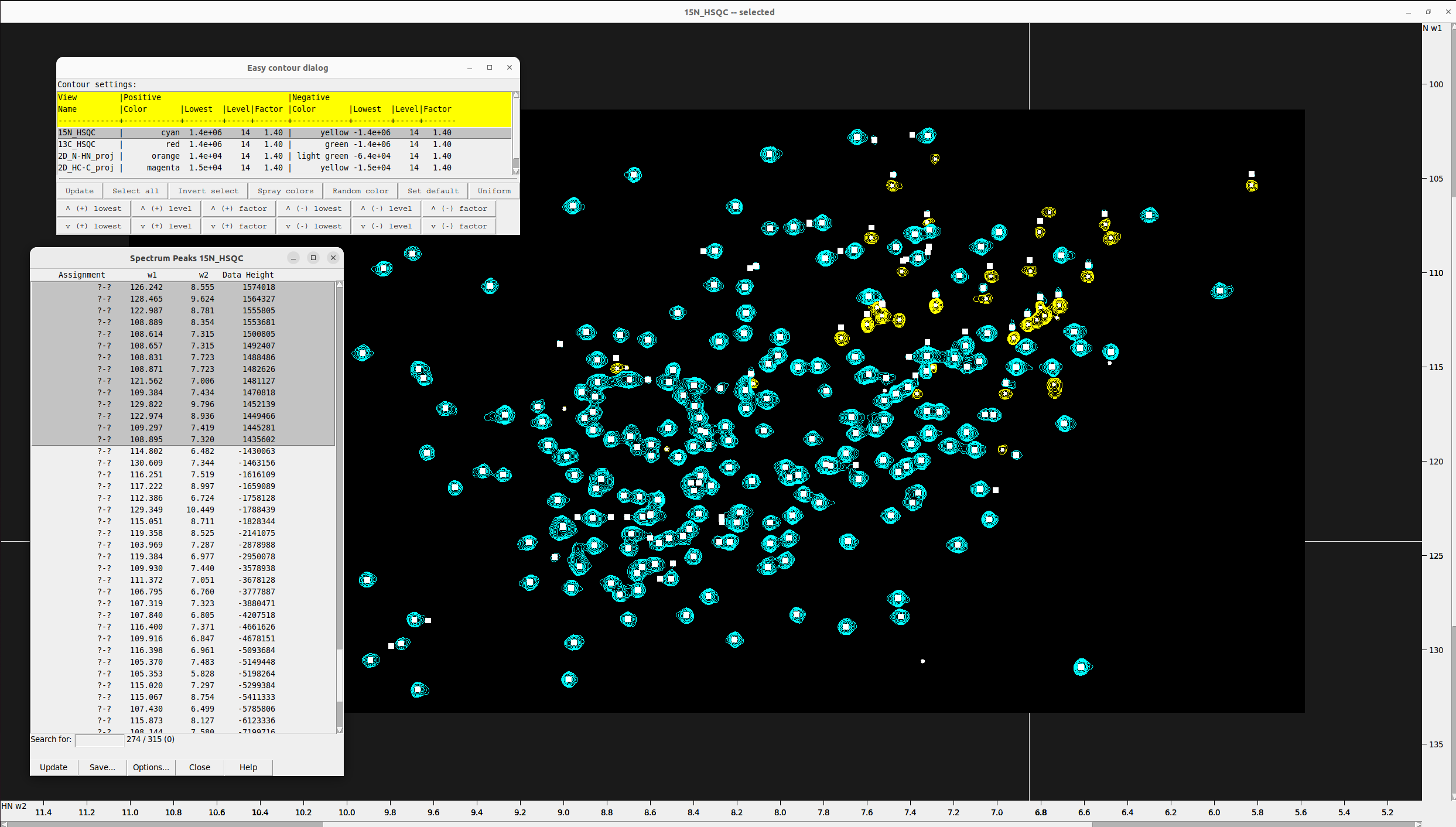
• Press lt to open the peak list and export the peak list from the 15N HSQC spectrum by saving it to a file.
• Press Ng to open the “Nucleate grid” plugin GUI, create and refine grid points for restricted peak picking as described below.

5.2 Optimizing Restricted Peak Picking for Higher Accuracy

For more accurate restricted peak picking, use the “Nucleate Grid” plugin in POKY. This tool helps generate artificial peaks in the form of a grid lattice, seeded from original peaks in your 2D reference spectra—in this context, from the 15N-HSQC and 13C-HSQC spectra.

How to install the “Nucleate grid” POKY plugin: copy the file nucleategrid.py to poky_linux/modules/poky and inside poky_linux/modules/poky/poky_site.py add the following line under ('restrictedpick','show_dialog')),: ` (‘Ng’, ‘Nucleate grid’, (‘nucleategrid’, ‘show_dialog’)),`.

The grid is generated starting from these reference (or “seed”) peaks and is expanded until an elliptical shape is formed, as defined by the parameters r1 and r2. You can also add spacing between grid points using the w1_step and w2_step padding parameters. To select the optimal r1 and r2 values for your spectra, focus on a few representative peaks and hit ms to measure their radius in both axes.

Once the artificial peaks are created, press lt to select and delete the low-intensity ones. This step refines the grid so that it covers only regions in the 2D spectra with high signal-to-noise ratios, as shown in the figures below.

You can then use all these peaks—including the real seed peaks and the newly generated artificial ones—for restricted peak picking. This helps capture more peaks in the target 4D NOESY spectrum, which is beneficial because 4D-GraFID can automatically handle noisy peaks and refine the selection using heuristic criteria. It’s better to capture more peaks at this stage to avoid missing real, informative inter-residual peaks that help build the NH-map. 4D-GraFID will remove the noise peaks automatically later.

---

5.3 Pick peaks in the 1H-13C HSQC

Repeat the same peak picking procedure for 1H-13C HSQC and create grid points for restricted peak picking.

5.4 Perform Restricted Peak Picking using 15N HSQC and 1H-13C HSQC as reference

Since this protein is large, we will perform restricted peak picking in two rounds.
This is necessary because the screen updates every time a picking cycle completes, and for large proteins, this eventually becomes terribly slow.

• First, select approximately half of the peaks in the 15N-HSQC.
• Press kr to open the Restricted Peak Picking window. Make sure you copied our enhanced plugin to your POKY distribution (see Prerequisites)!
• Activate the toggle options:
  • Use selected peaks only
  • Use tolerance values from note
• Under Find peaks, select the 4D NOESY spectrum.
• Under Using peaks in, select the 15N-HSQC.
• Click the Pick Peaks button.
• Once it finishes, repeat restricted peak picking, this time:
  • Set Using peaks in to the 13C-HSQC
  • Deactivate the toggle Use selected peaks only
  • Click the Select Peaks button.
• Then, switch to the 4D NOESY window, press Ip (capital i), and then the Delete button to remove all irrelevant peaks.
• The remaining peak list displayed on the HC-C plane of the 4D NOESY should now look clean.
• Press pa (select all), then NT, and write a word like matched to mark these peaks.

• Click Apply.

• Now go back to the 15N-HSQC window.
• Select the remaining half of the peaks.
• Open the Restricted Peak Picking window again.
  • Set Using peaks in to the 15N-HSQC.
  • Activate both toggle options:
    • Use selected peaks only
    • Use tolerance values from note
  • Click the Pick Peaks button.
• Change Using peaks in to the 13C-HSQC.
• Deactivate Use selected peaks only.
• Click Select Peaks.
• Switch to the 4D NOESY window, press NT, write the word matched, and click Apply.

⚠️ Important: Do not delete any peaks yet, as we did in the first round—otherwise, you will lose some of the peaks identified earlier.

• Press lt to display the pick list in the 4D spectrum.
• Click Options, sort the list by Note, activate the Note toggle, and click Apply.
• Our goal is to delete only those peaks that do not have a note. The good peaks are those with the word matched in the Note column.
• Use the Page Up and Page Down keyboard buttons to scroll quickly and select large portions of peaks without notes.
• Once a significant portion is selected, switch to the 4D NOESY window and press the Delete key to remove the selected irrelevant peaks.

💡 For large proteins with tens of thousands of peaks, it is recommended to delete them in two batches rather than all at once.

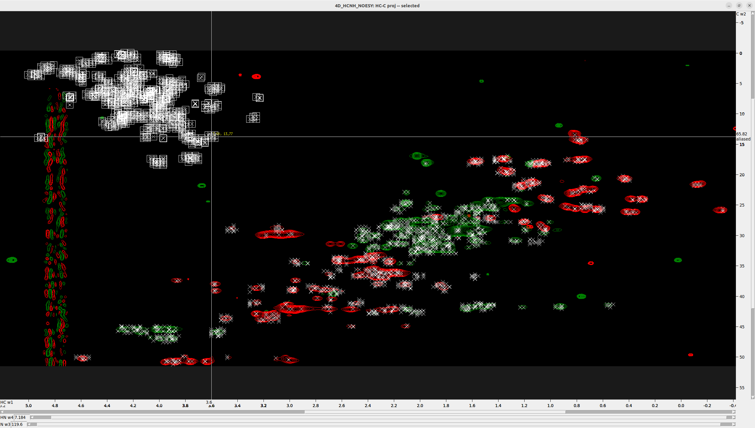
This is how the final peak selection on the HC-C plane of the 4D NOESY (overlaid on the 13C-HSQC for clarity) should look.

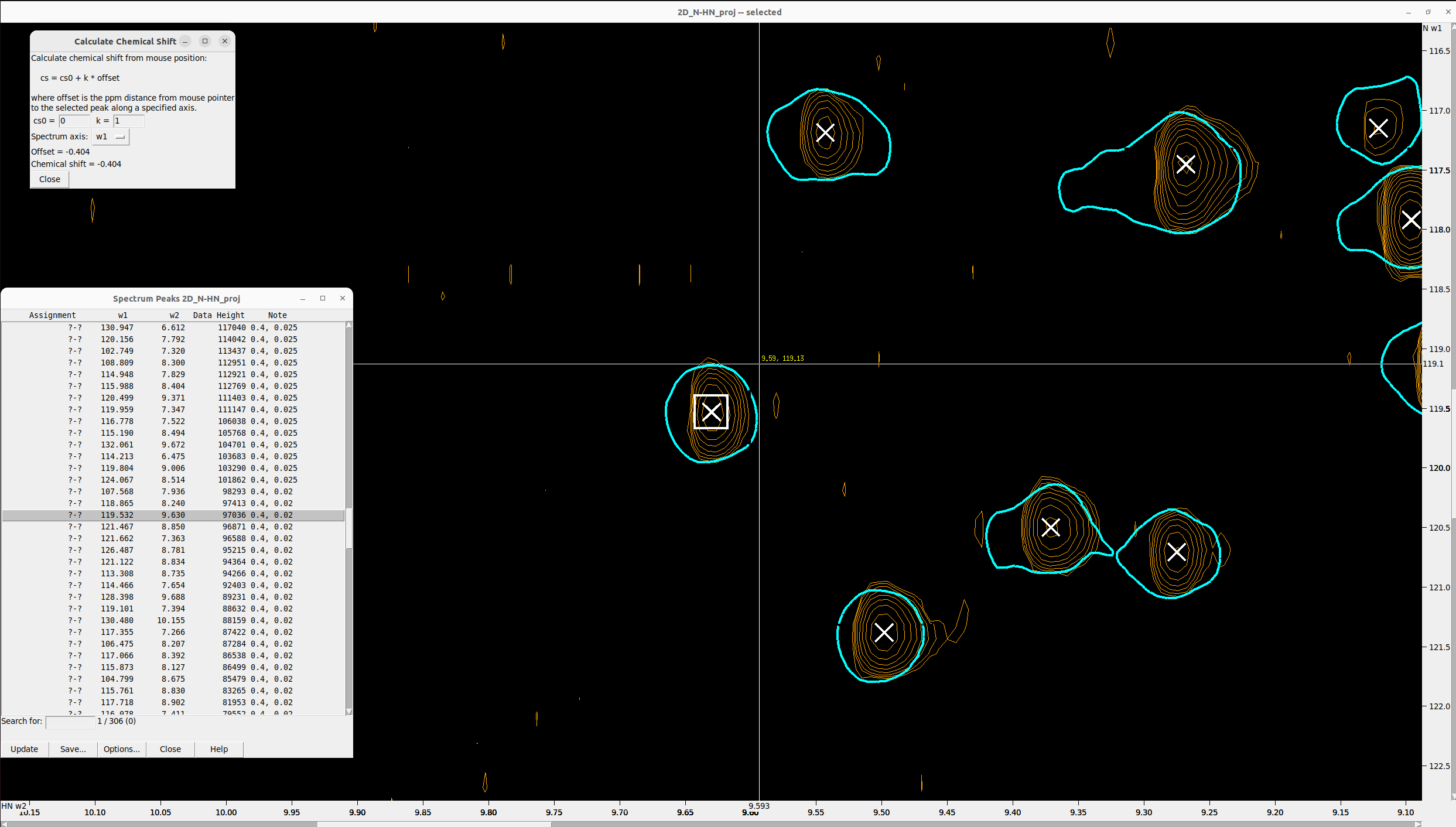
Step 6. Unalias/Unfold 4D Peaks (if necessary)

Next, we will perform unaliasing/unfolding of peaks - if there are any. For more details, please read the respective article.

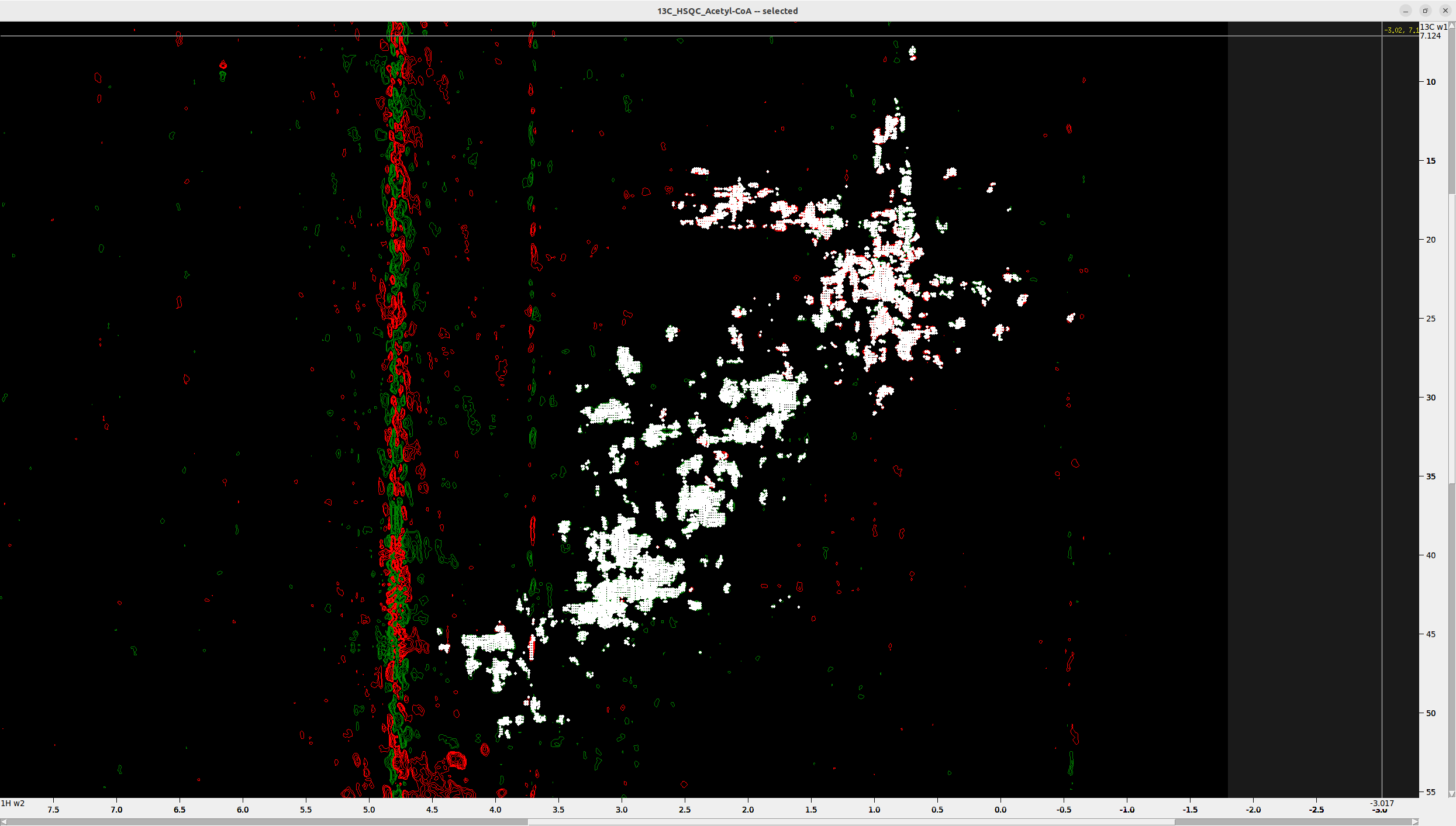
Aliased peaks usually occur in the ranges C < 25 ppm and HC > 3 ppm.

For demonstration, I show you the 4D spectrum of another protein, which has many aliased peaks that appear on top.

• Press F1 to switch to selection mode, select the aliased peaks, and then press a1 to unalias them along the C axis (W1).
• Hover over the aliased peaks and you will notice the word “aliased” appearing along the C axis (W1).

---

Step 7. Manual Refinement of 4D Peak List

Discard the 4D noise peaks using an S/N cutoff

• Hit st and in the text box “noise as median of” write 10000 or another high number.
• Click “Recompute” several times.
• If the “Estimated noise:” changes a lot, increase the “noise as median of” and repeat the process.
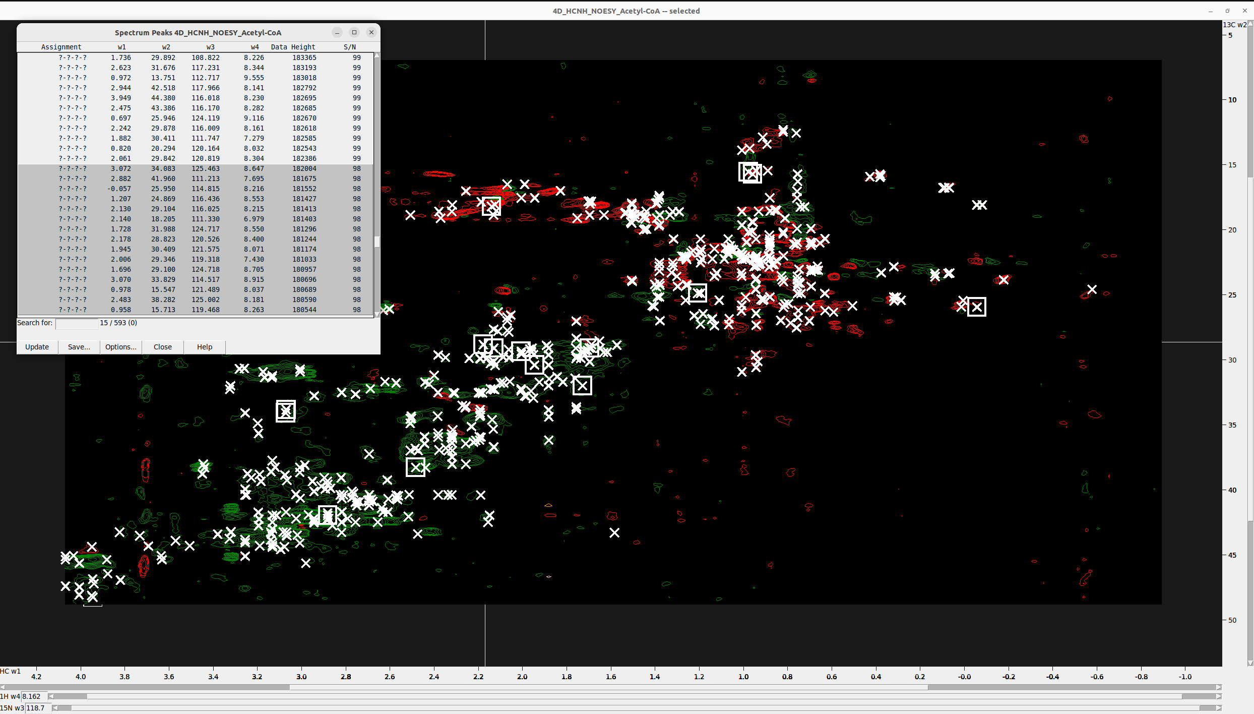
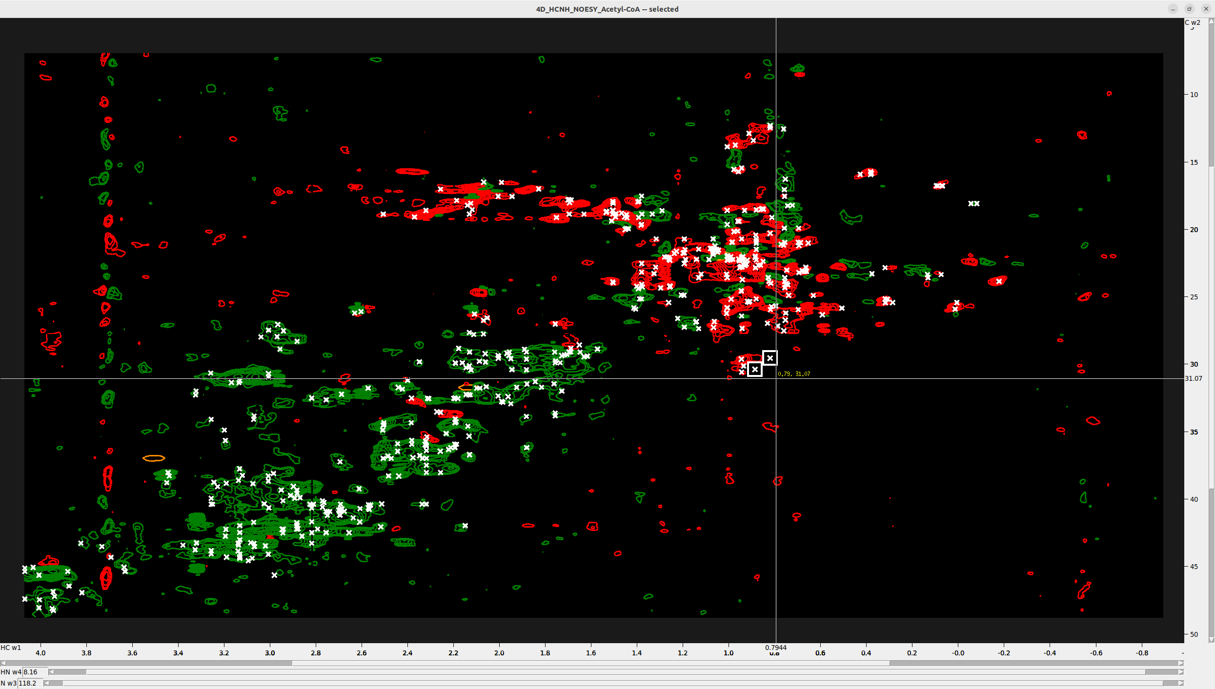
• Once you settle on an “Estimated noise:” value, open the peak list by hitting lt, display the S/N and sort by Data Height.
• Select all peaks with absolute S/N value less than the “Estimated noise:”, like in the Figure below, and delete them. For stricter peak picking, you can set the cutoff to 2x or 3x the “Estimated noise:”. Do not set the threshold high because 4D-GraFID can identify and remove the noise NOESY peaks automatically.

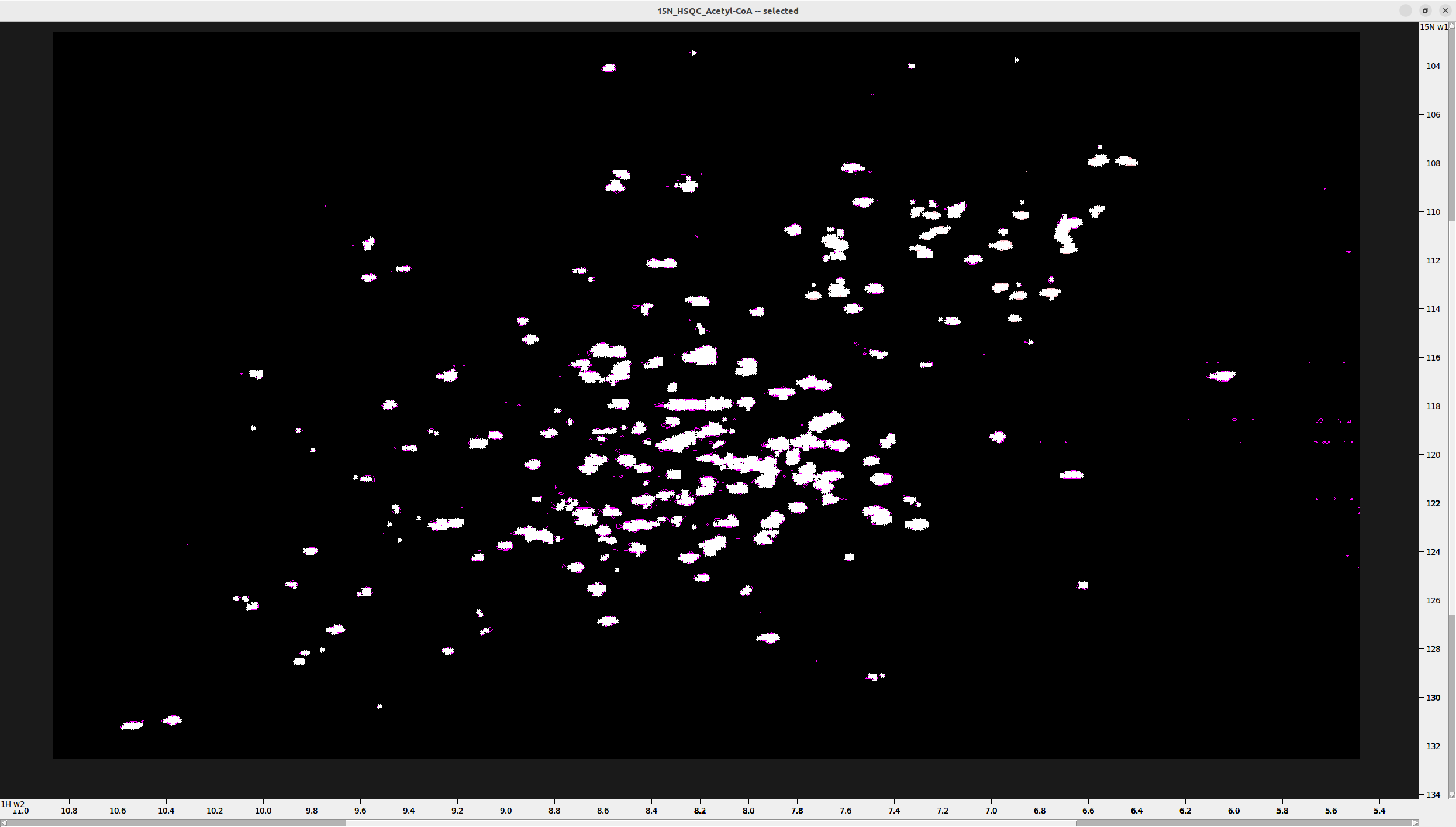
Discard the noise peaks using the 13C-HSQC and the 15N-HSQC

Next, we will manually inspect all the 4D peaks and remove those that are not located in density regions—neither of the 13C-HSQC nor of the 15N-HSQC.

• Type fo and load the 4D spectrum again, this time to a new window.
• In the new window double-click xr followed by xx to bring the N and HN axes into view.
• Adjust the view by pressing vt and increasing the aspect.
• Press vz, set the values to:
  • N and HN axes = 0
  • C and HC axes = 9999
  • Click Apply.
• You might need to adjust the peak sizes by typing oz.
• Hit ol and overlay:
  • First the 15N-HSQC onto the 4D
• Hit st and rename this window to 4D_HCNH_NOESY - 15N-HSQC

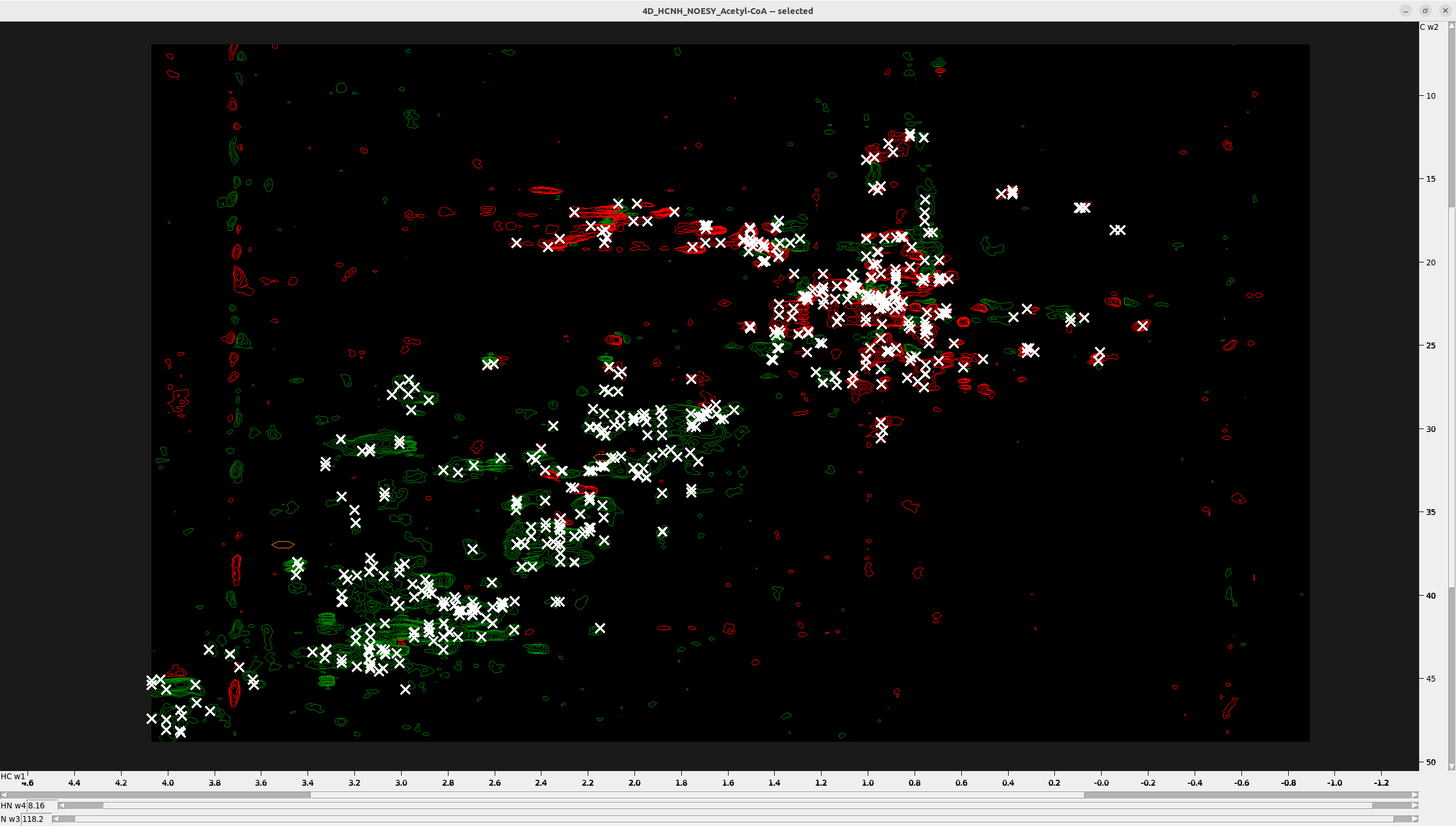
You should now have two different views of the 4D spectrum:

1. One showing the selected peaks on the HC-C plane
2. The other showing the selected peaks on the N-HN plane

What you must do next is manually inspect the peaks and delete those not in density regions. This requires a bit of intuition and a sharp eye. Unfortunately, it cannot be automated—it must be supervised manually by pressing st. Below are shown two obvious noise peaks on the HC-C plane view.

---

Step 8. Exporting Peak Lists for 4D-GraFID

8.1 Export Picked 4D Peaks

Go to the 4D peak list (type lt) and select the columns w1, w2, w3, w4, Data Height. Click Apply, then Save….

8.2 Enhance the 13C-HSQC peak list with multiplicity information (which C–H is methylene)

• Once you have finalized the peak list from the standard 13C-HSQC, export it to a file.
• Press fo and reopen the 13C ME-HSQC spectrum in a new window.
• Press st and rename that window to “refined 13C HSQC Peak List”.
• Hit rp, toggle on Auto detect dimensions and load the standard 13C-HSQC peak list.
• Verify that the aliased/folded peaks are unaliased/unfolded, just as on the standard 13C-HSQC spectrum (POKY does this automatically).
• Hit lt and through the “Options” display the “Data Height”.
• Export the updated peak list to a new file named standard_13C_HSQC_with_ME_peaks.list.

We follow this approach because the 13C ME-HSQC spectrum is very noisy, with large dispersion effects, meaning that the peak centers deviate from those identified in standard 13C-HSQC spectrum, which provides the maximum possible resolution and S/N. As such, we end with a near-complete aliphatic C-H peak list with information on whether a peak corresponds to a methylene group, which improves both accuracy and coverage for chemical shift assignment in 4D-GraFID.

8.3 Enhance the 15N-HSQC peak list with multiplicity information (which peak comes from N–H and which from N–H2)

Apply the previous trick but on the standard 15N-HSQC peak list using the 15N ME-HSQC spectrum. Export the new peak list to a file including the intensity column of 15N ME-HSQC, which tells which peaks originate from an N-H and which from an N-H2 group. This information is used by 4D-GraFID to identify the side-chain amide peaks.

---

Notes for Special Cases

Unaliasing Peaks in POKY
When you do restricted peak picking (kr) using as a reference peaks that have not been unaliased or unfolded, POKY will automatically check for possible aliased peaks. If the spectrum width of the reference 2D is larger than that of the target 3D/4D spectrum, POKY will find and mark the peaks in the 3D/4D as aliased.

However, BEWARE that when your reference peaks are unaliased or unfolded, POKY won’t match the correct peaks in the target spectrum unless they are also unalias/unfolded. It may catch some peaks but they will be irrelevant. Therefore, do not unalias/unfold the peaks in the 2D HC-C and N-HN projections! Do the unaliasing/unfolding directly on the 4D HCNH NOESY.

Below are examples of the 13C-HSQC spectra with aliased peaks (in yellow boxes):

Protein 1	Example 13C-HSQC - Protein 2

---

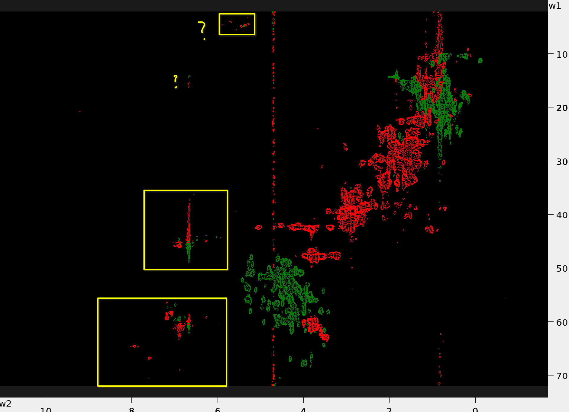Authors

• Thomas Evangelidis
• Ekaterina Burakova