Phase Correction in 3D Protein Spectra
In the 3D spectrum, phase correction is done for every dimension individually. SOLUTION 1 is only for the direct (F3) dimension, while SOLUTION 2 is for every dimension. I strongly recommend using them in combination.
Table of contents
Tested environment:
- Topspin 4.4.0 with commercial license for NUS processing
- OS: AlmaLinux 9 (as an Oracle virtual machine)
- 20 CPU cores, 120 GB of RAM.
SOLUTION 1: Phase-Correct the 1st FID (F3)
The 1st (strongest) FID always corresponds to the direct (F3) dimension. Therefore, you cannot phase F2 and F3 with this solution.
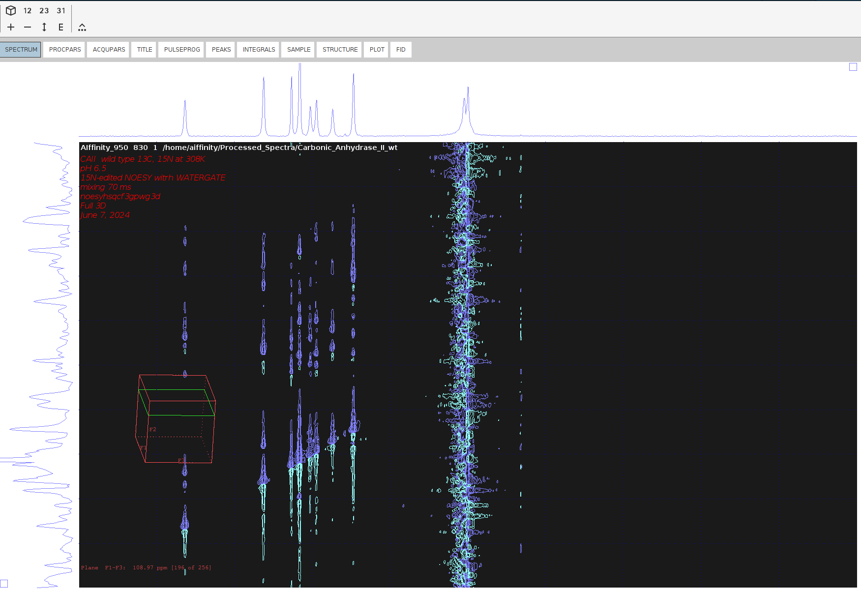
Example Data: N-edited 3D NOESY of Carbonic Anhydrase 2 (29 kDa)
- Reset all phase values to
0:Important: Look at the bottom of the pulse program to find the correct PHC0 and PHC1 values of F1-F3 - if there are any.
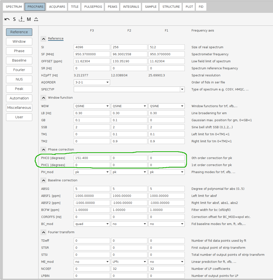
- Set all phase values to zero with the following commands:
3 PHC0 0 3 PHC1 0 2 PHC0 0 2 PHC1 0 1 PHC0 0 1 PHC1 0 - Reset spectrum truncation boundaries with the following commands:
3 TDeff 0 2 TDeff 0 1 TDeff 0 3 STSR 0 2 STSR 0 1 STSR 0 3 STSI 0 2 STSI 0 1 STSI 0 - You may want to increase the points in any dimension (
SI) by x2 or x4 times (zero filling) to enhance resolution. Ensure that all SI values are powers of 2 (e.g., 1024, 2048, etc.).
- Set all phase values to zero with the following commands:
Note: Linear Prediction is beneficial when only a few points have been recorded in a dimension, otherwise it may be detrimental and thus must be turned off.
- Navigate to
PROCPARS -> FOURIERand set the parameter ME_mod tonofor all dimensions except those that only a few points are recorded. In this example only F2 (C), which had only64points, and thus I quadrupled them.
- Extract the 1st FID:
- Open the raw 3D spectrum and run
rser eao 1to extract the 1st FID followed byftto switch to the frequency domain. Note that for other spectra, theeaoargument may not be appropriate (see when to userser 1and whenrser eao 1). - Alternatively, you can create a macro using the command
edmac qfp. - In the editor that opens, write the following commands to save and process the spectrum:
qsin fp - Run the command
qfp. - In the pop-up window, set
1atFIDand2atPROCNO. - Issue twice
.grto display denser grid lines.
- Open the raw 3D spectrum and run
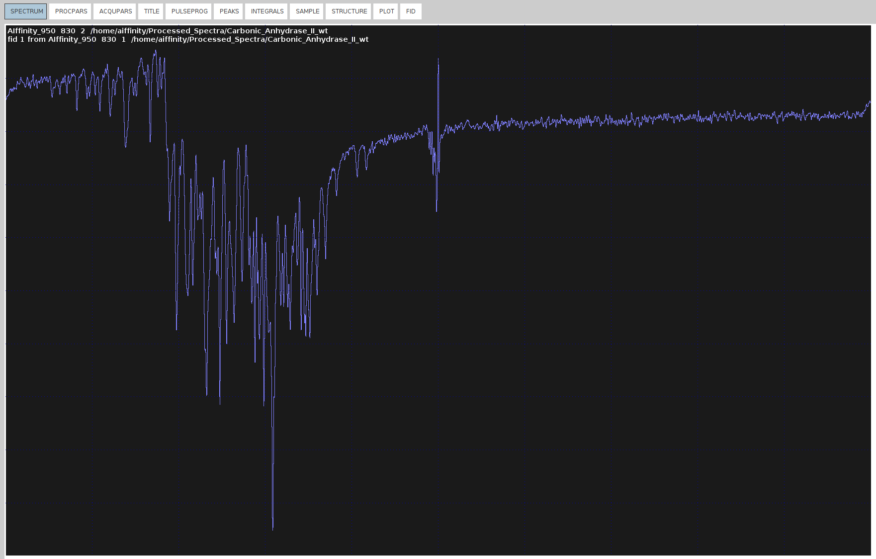
- Phase Correction:
- Try first the automated 0th order phase correction with
apk0that will try to create an entirely absorptive lineshape in the spectrum. - If you are not entirely satisfied with the automatic phasing, enter
.phfor manual phase correction. Set the pivot line (right mouse click) near the right limit to modify onlyPHC0, notPHC1.Note: Adjusting
PHC1(1st order correction) has minimal effect on frequencies near the pivot and no effect onPHC0. - Shift baseline to bottom with
.sdand adjust its position with the arrow icons. - Adjust only
PHC0(0th order correction) so the FID line extends straightly and the highest peaks point upwards.Note: Avoid using automatic phasing (
apkand its variants) as it generally doesn’t work well.
- Try first the automated 0th order phase correction with
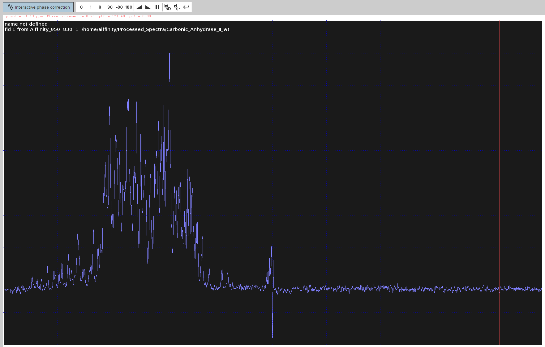
- Save and Apply PHC0:
- Note down the optimal
PHC0value (e.g.,151.40degrees). Click the Save-disk nD icon to copy the values to the 3D spectrum, then click the Return icon. Double-click the processed 3D spectrum and ensure allPHC0andPHC1values except for F3(PHC0) are still set to0.
- Note: sometimes when the data was moved around, the Save-disk 3D button will complain on non-existing paths and wwwill not work. In those cases, one has to transfer the phasing coefficients manually.
- Note down the optimal
- Initiate NUS-reconstruction:
- Execute
FnTYPE. If this option is not set tonon-uniform samplingthen you can safely useftnd 0 nusftor justft3dinstead offtnd 0to skip the NUS-reconstruction in all relevant steps from this point on. But even if you runftnd 0, Topspin will recognize it by itself and skip the otherwise tedious NUS-reconstruction. - Select the
csmethod within the NUS section of PROCPARS window or simply execute3 Mdd_mod cs. - Execute the command
ftnd 0for Fourier transformation and NUS reconstruction - it shouldn’t last long in the 3D spectrum. This step helps in visualizing the spectrum and deciding on the dimensions to truncate.
- Execute
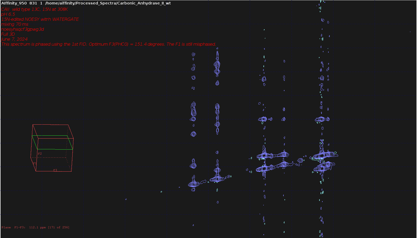
- Check Visually the NUS-reconstructed Spectrum:
- Click on the
23icon and navigate the F2-F3 plane by holding left-mouse button on the double arrow icon and dragging your mouse. You will notice that there are no antiphase peak components in the F3 dimension.
- Click on the
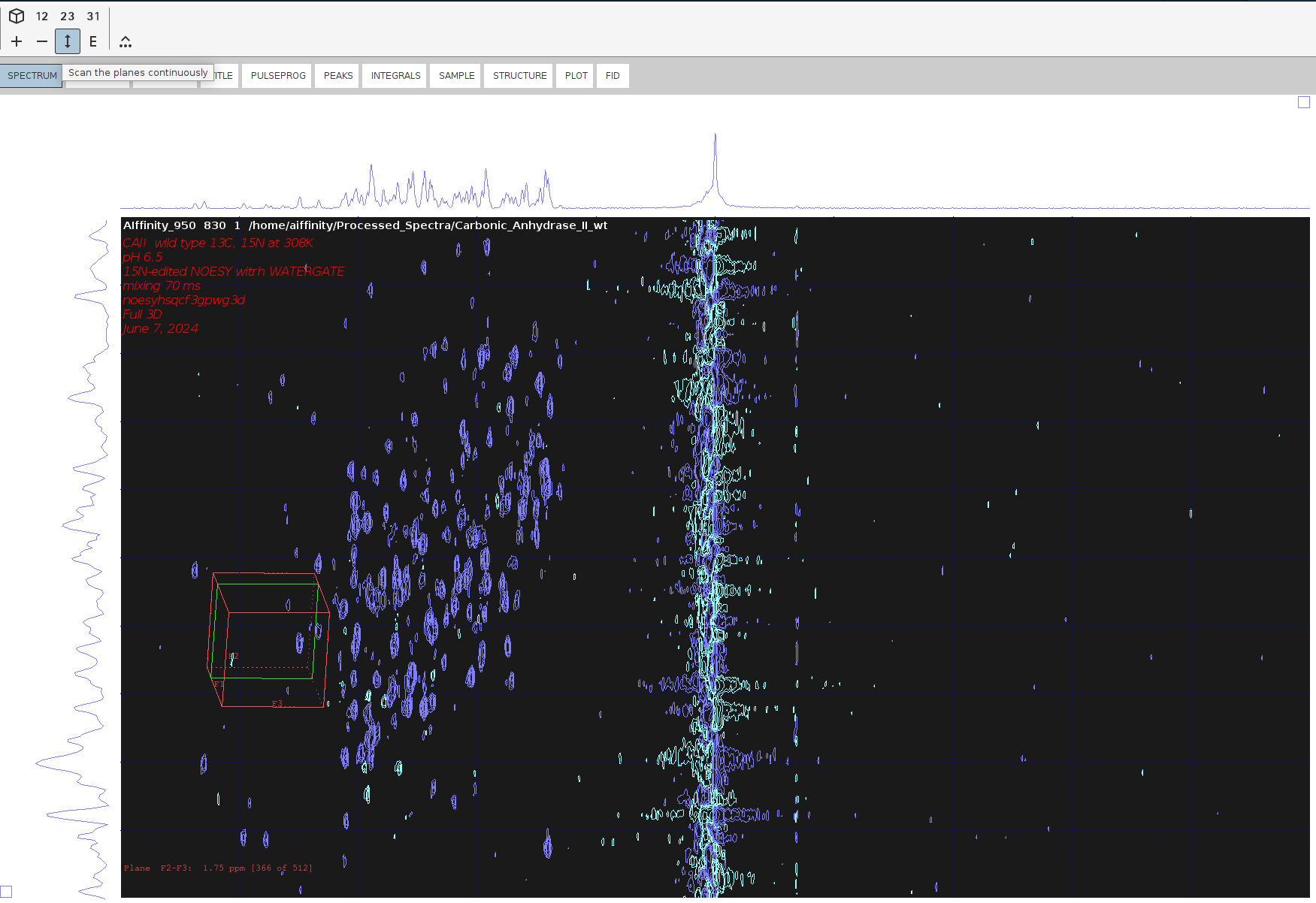
- Do the same for the F3-F1 plane by clicking on the 31 icon. There are plenty of antiphase peaks in the F1 dimension, which means that the spectrum needs additional phasing.
SOLUTION 2: Phase-Correct the F2-F3 sum projection of the 3D Spectrum.
Summary of Commands and Steps
- Reset all phase values to
0:- Like step 1 in SOLUTION 1.
- Initiate Fourier Transform with zero phase values:
- Like step 5 in SOLUTION 2.
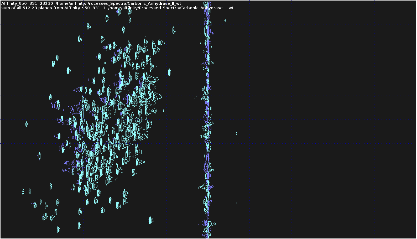
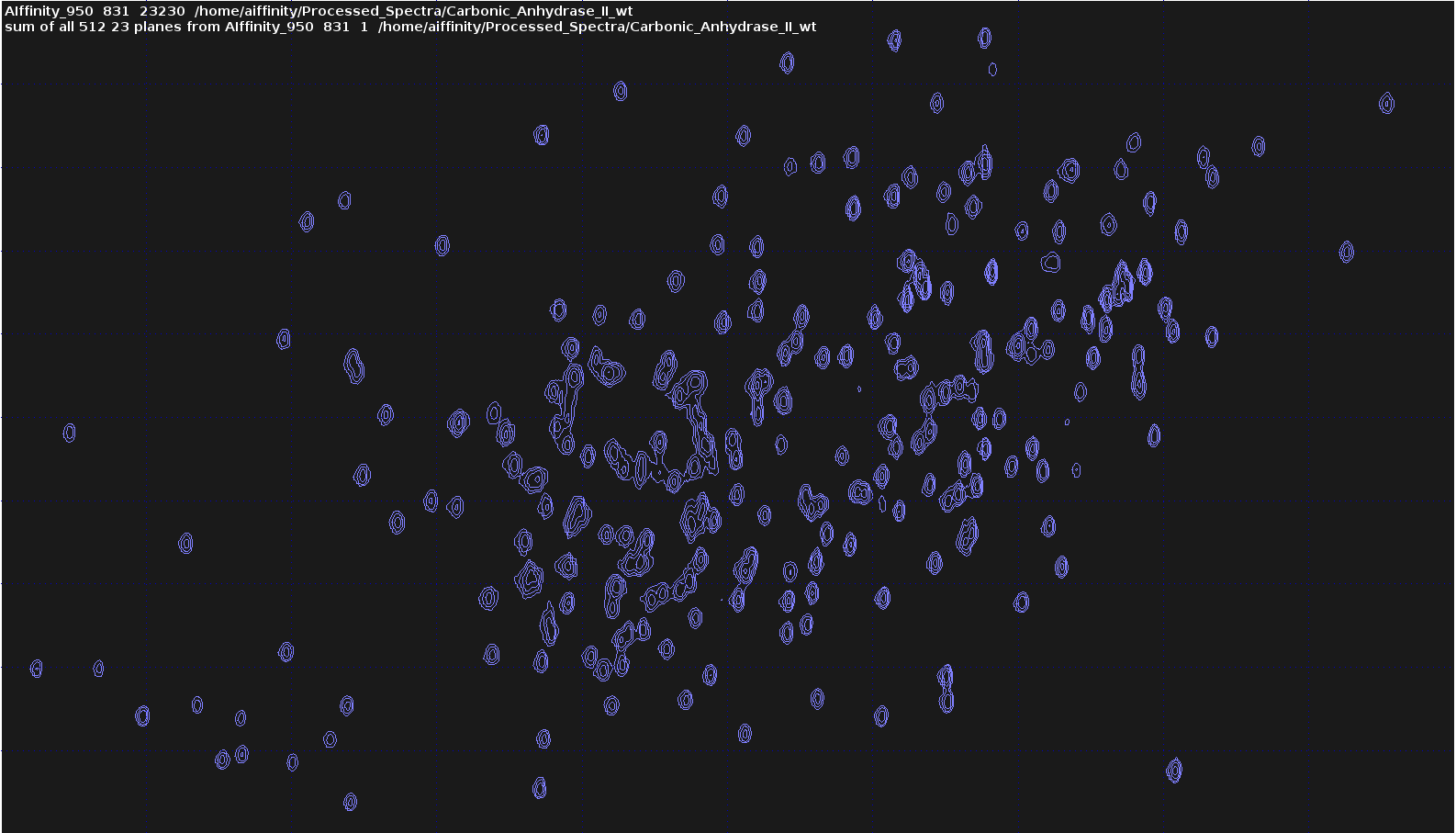
- Create the Sum Projection of F2-F3:
- Issue the following command to create the sum projection of F2-F3 (
N-HN):sumpl 23 all all 23230
- Issue the following command to create the sum projection of F2-F3 (
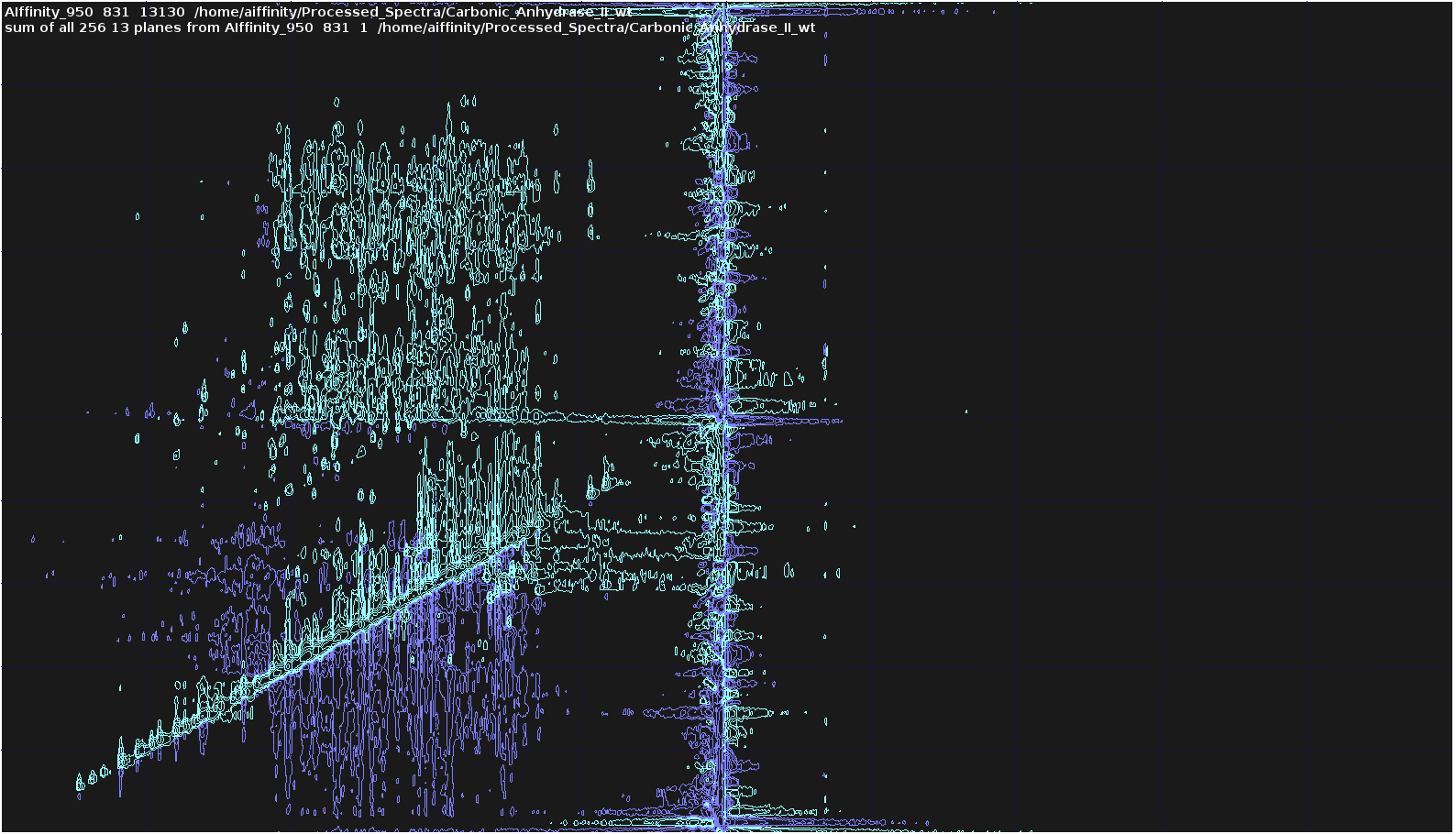
- Switch Back to the 3D Spectrum and the following command to create the sum projection of F1-F3 (
H-HN):sumpl 13 all all 13130
- Visualization and Dimension Truncation:
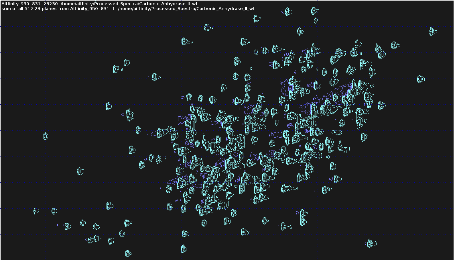
- Open the
23sum projection. The vertical line in the center represent water signal; the pulse sequences are designed to be symmetrical ensuring that the space before and after the water line is the same. - Zoom in by selecting the region of interest (RIO).
- Open the
- Right-click anywhere on the spectrum and then select
Save Display Region To -> Parameters STSR/STSI (used by strip ft). After this, the boundaries of the ROI will appear inSTSRandSTSIparameters under thePROCPARStab. - Right-click again anywhere on the spectrum and this time select
Save Display Region To ->
Parameters ABSF1/2 (e.g. used by 'absf, apkf')
. This is to ensure that the baseline correction takes place downfield (to the left) of the water line (~4.5 ppminHN) to avoid filling the spectrum with noise. - Transfer manually these values to the respective parameters of the 3D spectrum.
- Switch back to the 23 sum projection and issue the following commands:
1 ABSF1 1000
1 ABSF2 -1000
1 BC_mod no
2 BC_mod qpol
2 SSB 2.2
- These commands have the following effects:
- Leave the default
ABSF1andABSF2values in theNdimension. - Select the
qpolpolynomial function sinceqfilsuppresses water very aggressively and is not recommended for theN-HNspectrum. - Set
BC_modtonoin theNdimension due to its sensitivity to the polynomial. - Set the
SSBof the direct dimension to2.2for further resolution.
- Leave the default
- Execute
xfbfollowed byabs2andabs1for baseline correction. This will remove the irrelevantHNshift region, including the water line, while keeping only the ROI. It will also result in sharper and better-resolved peaks due to zero filling and increasedSSB.
- Repeat the same procedure for the
13sum projection.
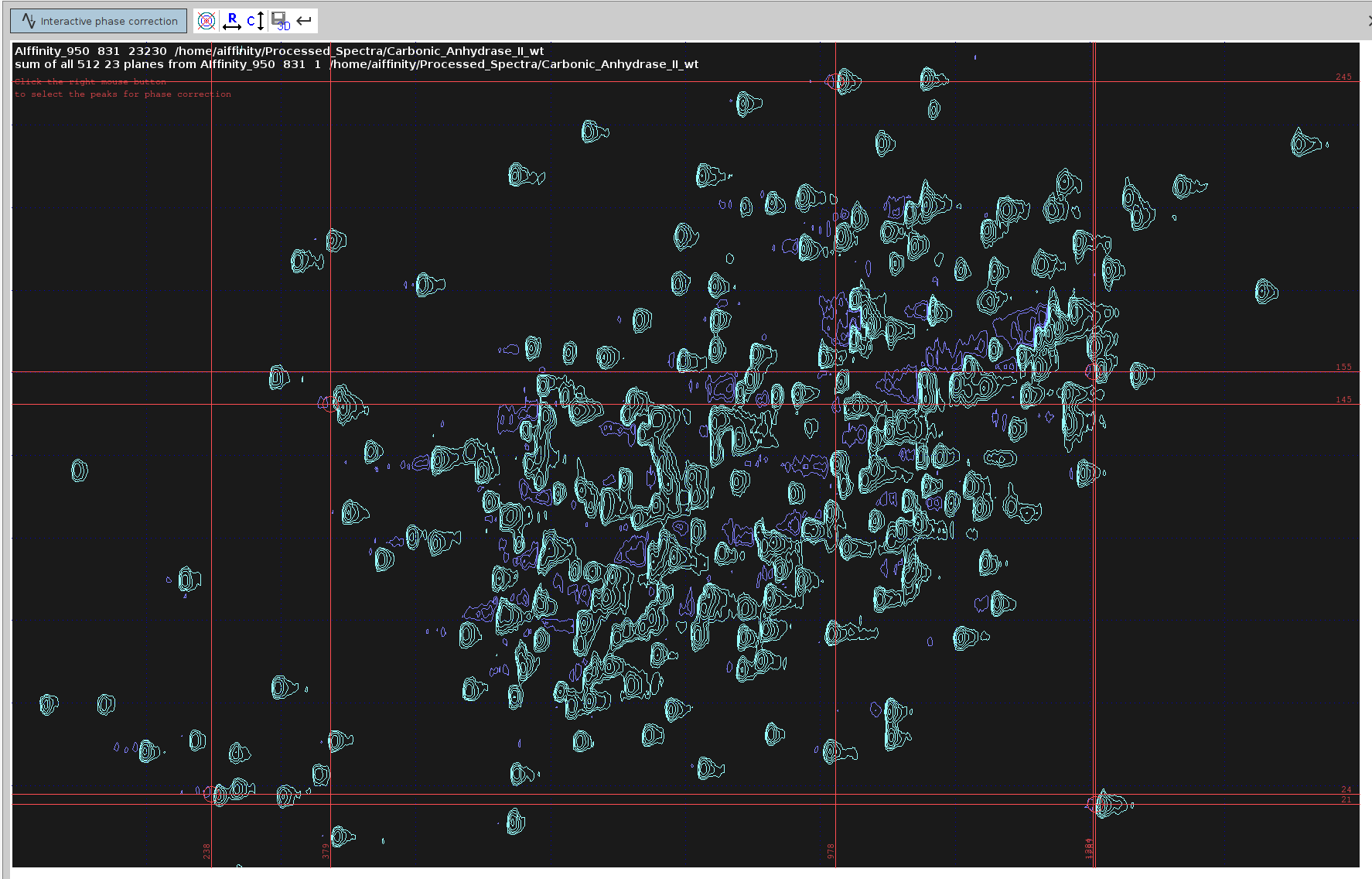
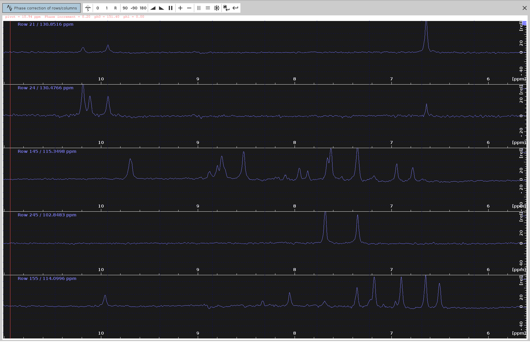
- Prepare for Manual Phase Correction in the F2 dimension:
- Enter
.phfor manual phase correction. - Look for peaks that have an anti-phase component in the F2 dimension.
- Place the cursor between the centers of these two peaks. Ensure the cursor is along the line connecting their centers.
- Right-click and select “Add”.
- Enter
- Try to select misphased peaks that cover the span of the whole spectrum; 4 or 5 peaks should suffice.
- Enter Phase Correction Mode:
- Click on the icon with the letter “R” to enter phase correction mode for the rows, which correspond to the
F2 (
HN) dimension in the23sum projection.
- Click on the icon with the letter “R” to enter phase correction mode for the rows, which correspond to the
F2 (
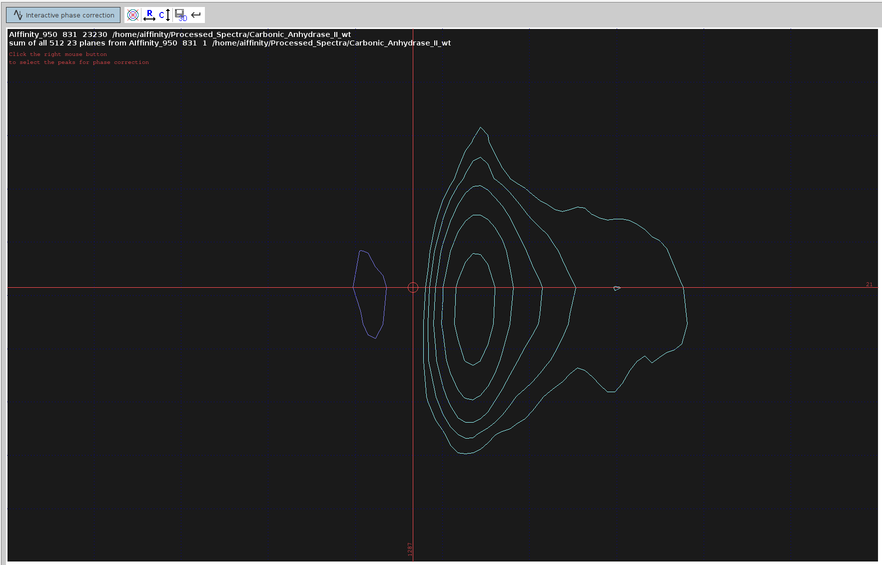
- Set the Pivot Point:
- Right-click at the left limit of the screen and select “Set Pivot”.
- Place the pivot point away from the peaks to avoid hiding the frequencies we want to phase.
- Note: Only the
PHC0value will be adjusted, notPHC1, so the pivot point will not be used.
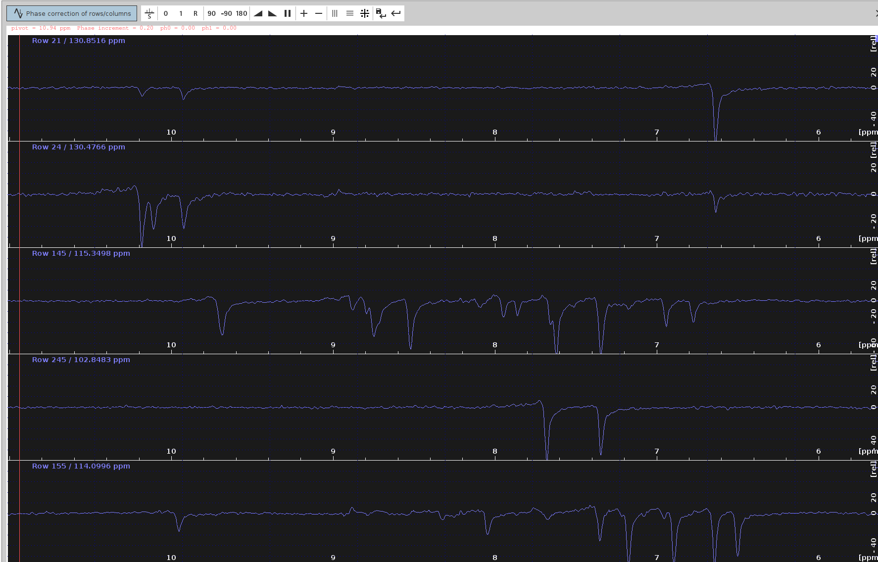
- Adjust the Phase:
- Left-button press on the “0” icon and drag your mouse until the strongest signals appear at the top part of each panel.
- Ensure the frequency lines from end to end look straight and balanced.
- Save the PHC0 Value:
- Note down the optimal
PHC0value (e.g.,151.40degrees) and click on the “Save-disk” icon to save the selectedPHC0value to the23sum projection spectrum. - Click the Save-disk nD icon to copy the
PHC0value to the 3D spectrum. - Then click the Return icon.
- Note down the optimal
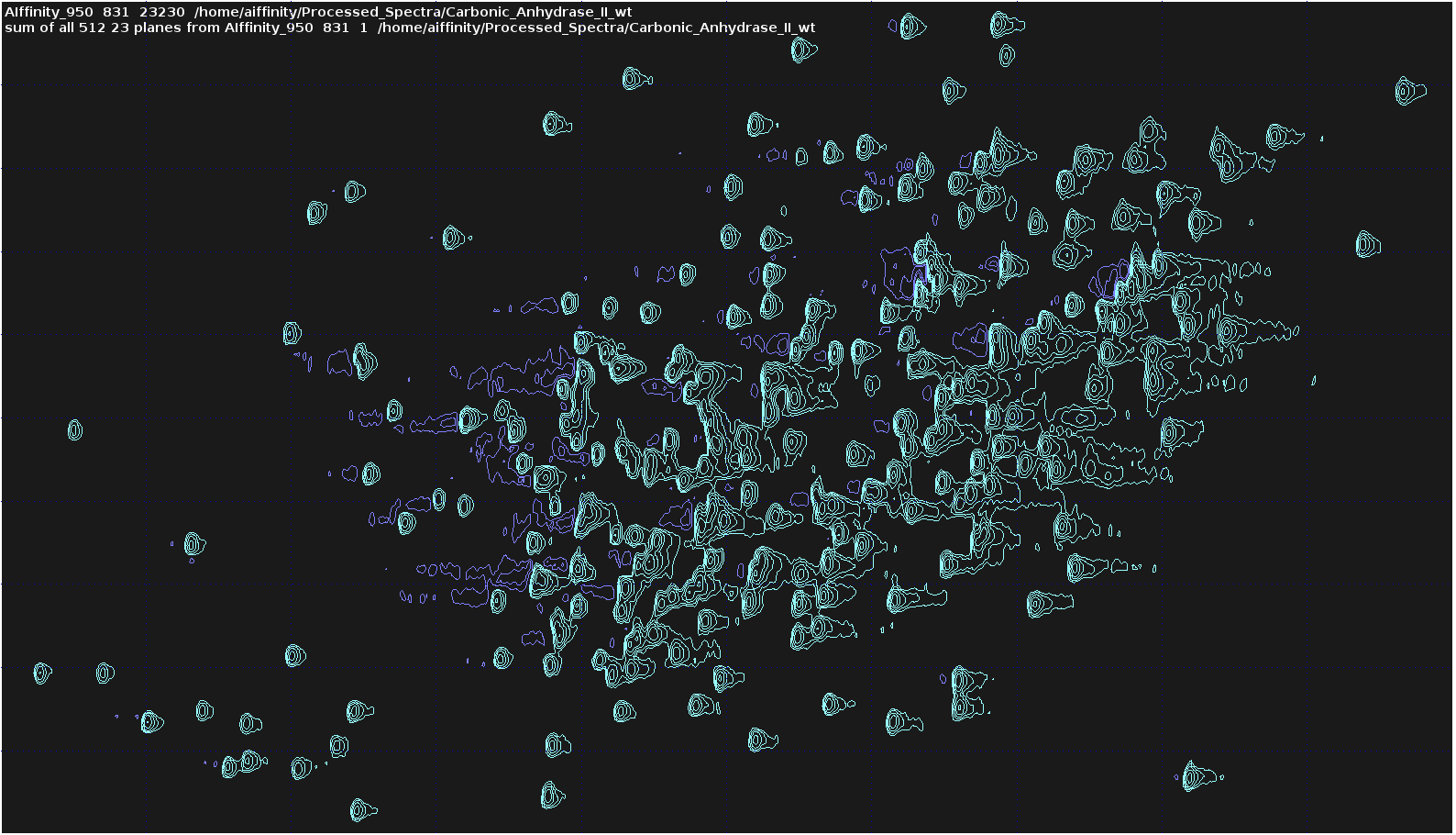
- Verify the Phase-Corrected Spectrum:
- The phase-corrected
23sum projection should now appear without any anti-phase peak components.
- The phase-corrected
- Save and Apply PHC0 to 3D:
- Switch to the 3D spectrum and run
ft3dfor FT and phase correction with the values you provided.
- Switch to the 3D spectrum and run
- Review and Adjust Peaks in 3D View:
- Return to the 3D view to review the changes by clicking the cube icon.
- Click on the /8 icon to display the peaks. Adjust the contour levels with your mouse.
- Click on the aim icon to switch to 2D plane view and then to
23. Navigate through different planes using the up and down arrows icon. Identify a plane where peak phases are unsatisfactory. In this example, I couldn’t find a plane containing misphased peaks, but you got my point.
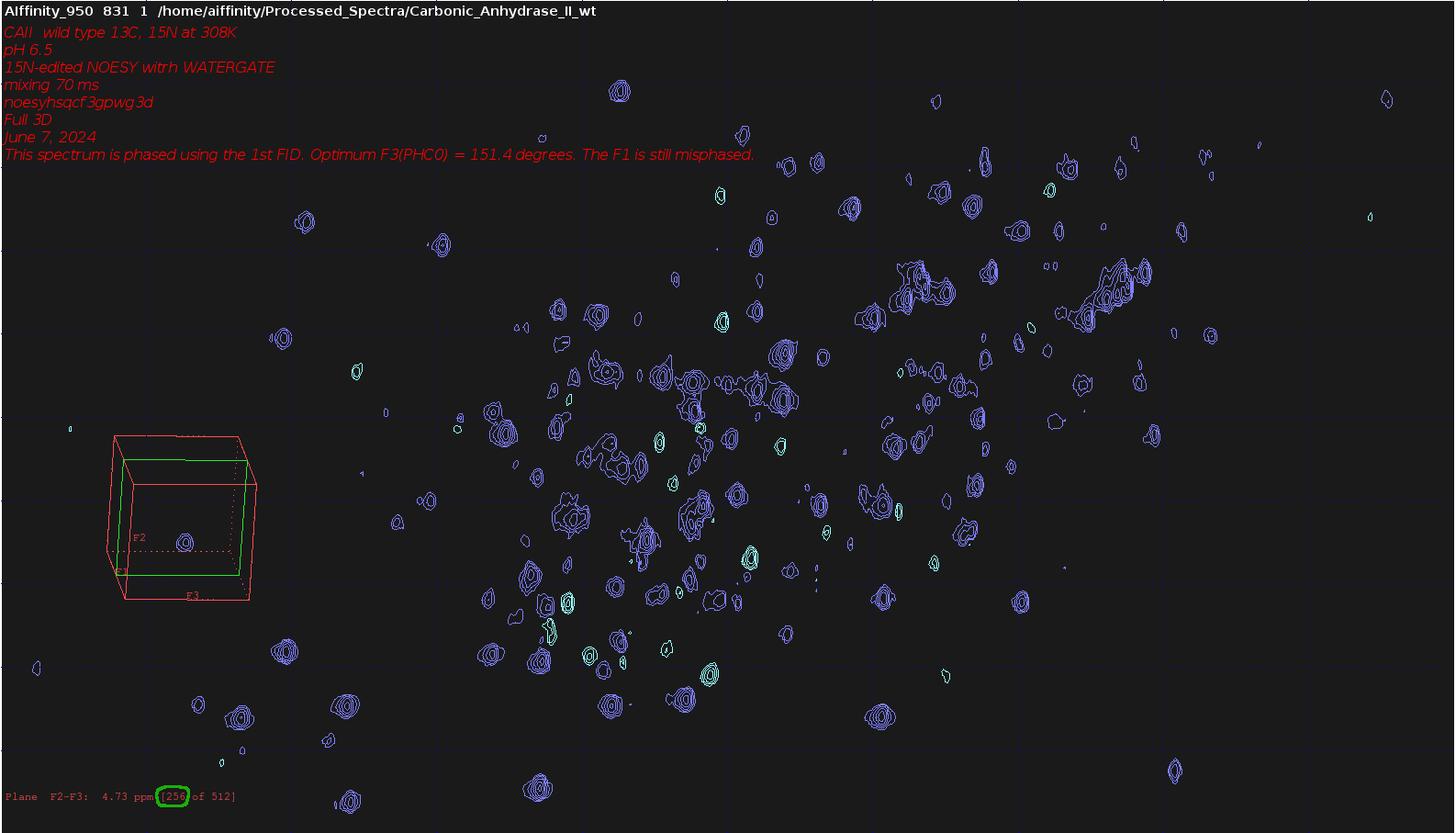
- Extract and Process a Specific Plane:
- Execute
sliceto extract the problematic plane. - A window will ask for the plane number (displayed at the bottom left in red letters; marked with green circle).
Enter a Destination PROCNO, e.g.
23265.
- Execute
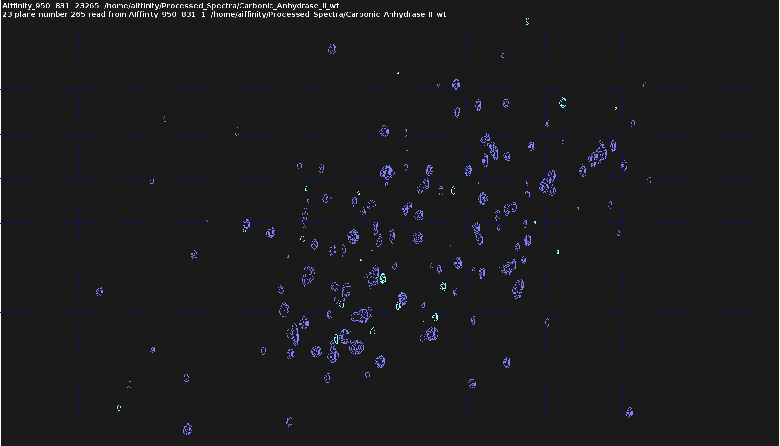
- Reconstruct Imaginary Dimension for Further Phase Correction:
- Use
xht1followed byxht2or navigate through the menuAdvanced -> Special Transforms -> Hilbert in F1and thenHilbert in F2to reconstruct the imaginary dimensions.
- Use
Note: Files like
3rrrrepresent the spectrum in real space, whereas files such as3iri,3irr,3rir,3iir, and3iiicontain at least one imaginary dimension. Correspondingly, the commandslicecreated a file2rrin the23265folder. The Hilbert transformation created the files with imaginary parts: 2ri, 2ir, and 2ii.
- Repeat steps 5-14 until you are satisfied with the phases of the F3 and F2 dimensions in the 3D spectrum.
- Repeat steps 5-14 for the
13sum projection until you are satisfied with the phases of the F1 dimension, too. There were no misphased planes in F1-F3 planes after phase correction. I just provide the most “weird-looking” one below for demonstration:
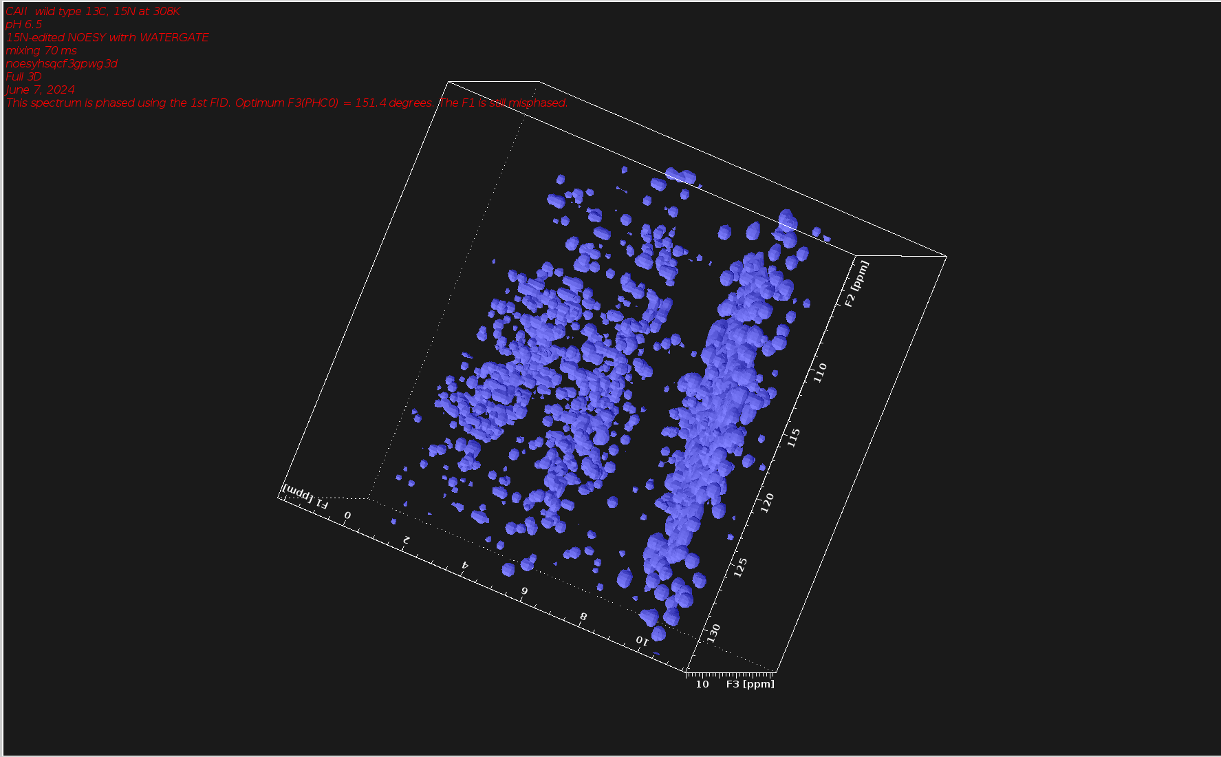
- The optimum phase values I found for this example were
F3(PHC0)=151.40andF1(PHC0)=-42.60and the 3D spectrum looks like this, without any visible negative signals:
Baseline Correction
- Increase FID Dimensions:
- Increase FID dimensions by x2, maximum x3 (e.g., if the dimension size is 60).
- Set Baseline:
3 BC_mod spol- Choose a baseline where there are no peaks. In the proton dimension, set
ABSF1 -> 9.0 ppmandABSF2 -> -4.0 ppm.
- Fourier Transform:
- Perform Fourier transform with
ft3d.
- Perform Fourier transform with
- Contour Level Adjustment:
- Click on the hill icon, set contour level sign to positive, Level increment to 1.2, and the number of levels to 30.
- Navigate and Adjust Peaks:
- Navigate in depth (F2 dimension) by clicking the + icon until you reach two overlapping peaks.
- Note down the plane number (e.g., 27/256).
- Iterate with different FID sizes, window functions, and linear predictions until the peaks separate. Do not apply linear prediction on the proton dimension because many points are acquired, but it can be done in the indirect dimension. Avoid overdoing it.
- Baseline Correction:
- Perform baseline correction with the commands:
tabs1 tabs3 - This corrects the baseline in F1 and F3 dimensions.
- Perform baseline correction with the commands:
Authors
- Thomas Evangelidis