How to Set Up a ¹H–¹⁵N HSQC Experiment in TopSpin

This tutorial walks you through every step—from loading your sample to fine-tuning shims and measuring signal-to-noise—so you can acquire high-quality HSQC data and compare the classic and BEST-HSQC variants. There is another tutorial based on a workshop, which will be eventually merged to this one.

---

1. Prepare a New Experiment Folder

1. Copy a previously calibrated ¹H experiment
   • In TopSpin, select an earlier proton pulse-calibration experiment (e.g. zg) and press new.
   • Create a new dataset and copy the parameters into it.
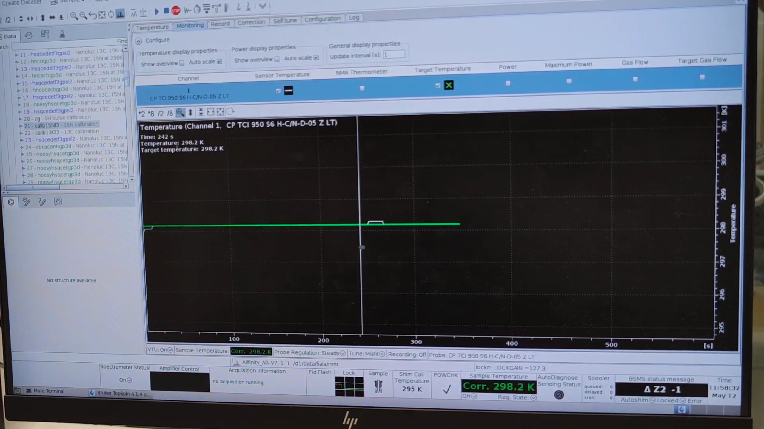
2. Set the temperature
   • Press edte and enter the desired temperature.

3. Insert the sample into the spectrometer.

4. Lock on the solvent
   • Press lock, choose the correct solvent (e.g. H2O+D2O), and wait ≈ 10 min for temperature stabilization.

Tip: While the sample equilibrates, you can start configuring the HSQC experiment.

---

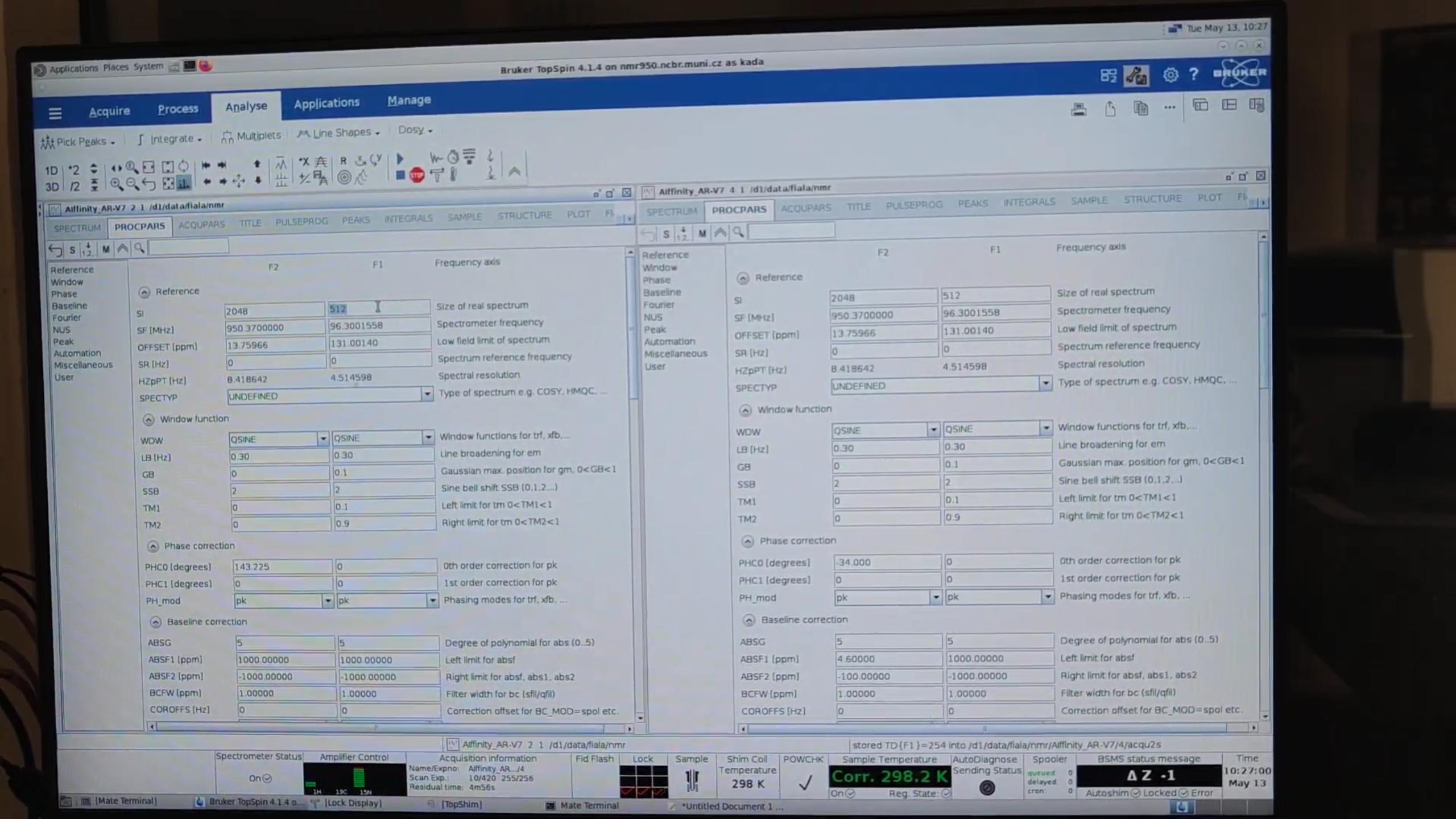
2. Load and Configure the HSQC Pulse Program

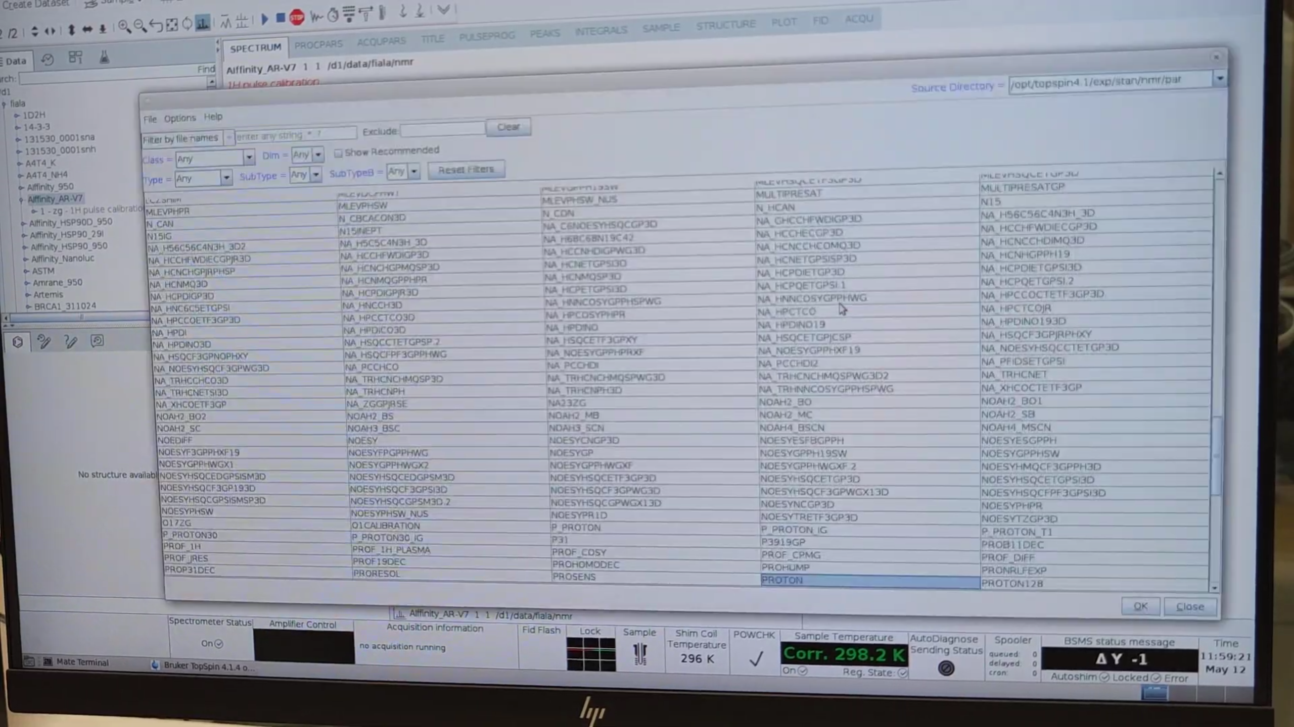
1. Press new → Read parameter set → choose an HSQC sequence (e.g. HSQCETF3FGPSI).
2. Select Execute getprosol to import pulse-length/power values.

3. Enter a short description under Title and click OK.

4. Verify acquisition channels
   • Press edasp.
5. Set basic parameters
   • Press eda and adjust
     • SW (spectral width)
     • O1P (reference offset)
     • AQ (acquisition time)
     • TD / DS / NS as needed for total experiment time (expt).

---

3. Probe Tuning & Matching

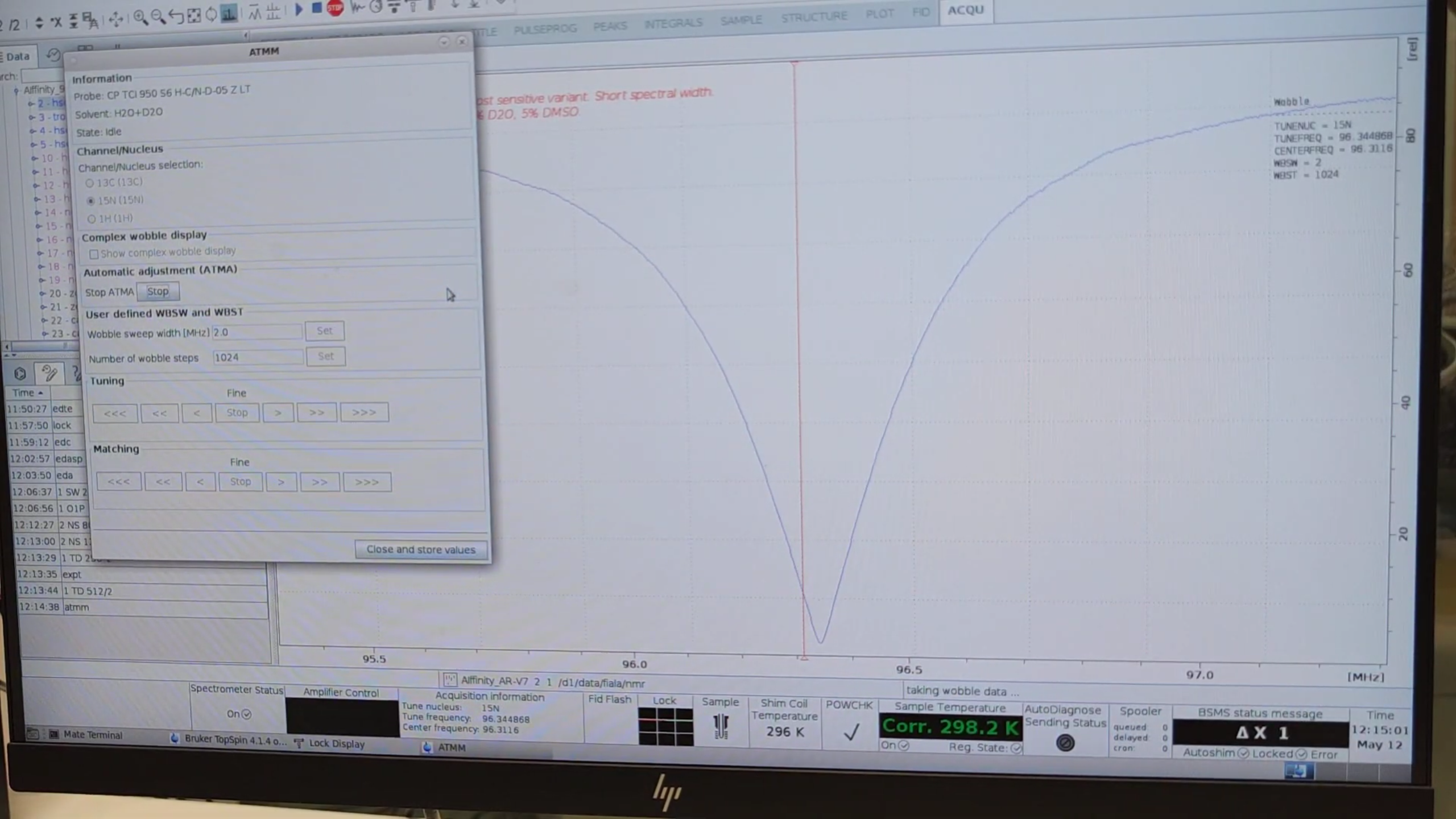
1. Press atmm (manual tune/match).
2. Select 15N, click Start, then repeat for 1H.

3. When automatic tuning finishes, switch to manual mode and center the minima on both channels.

4. Press loopadj to refine lock parameters.

---

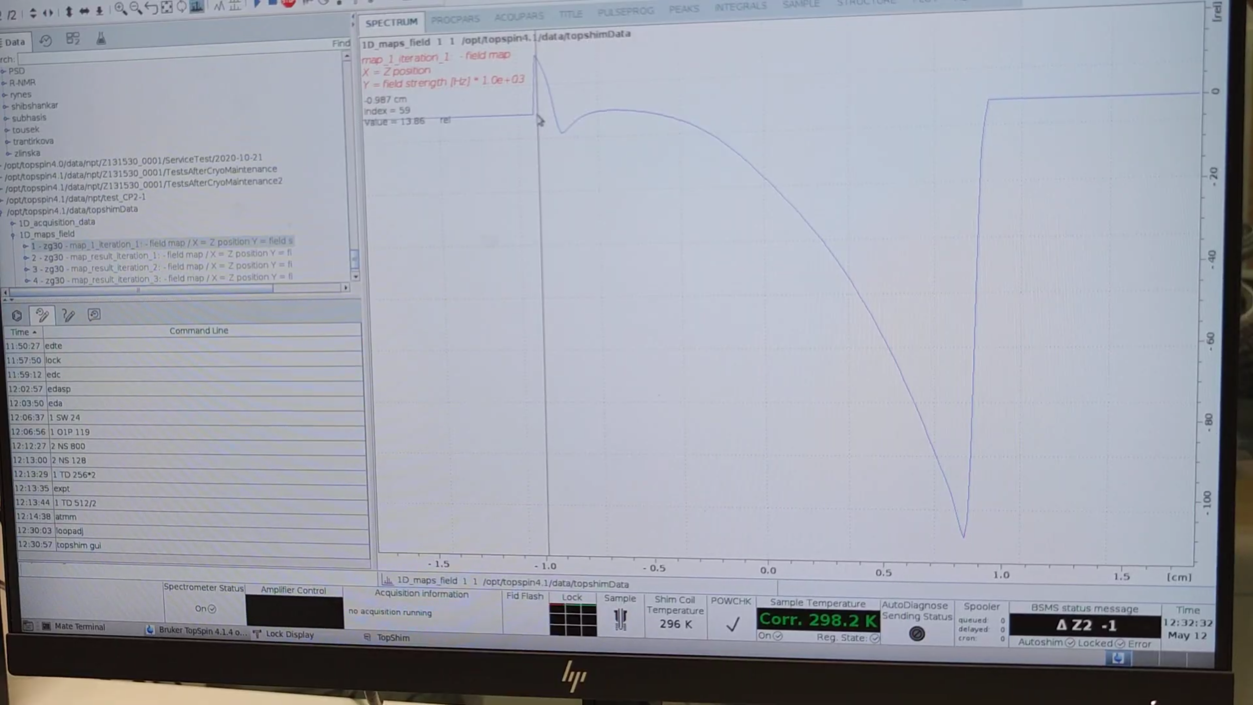
4. Automated Shimming (Shigemi Tube)

1. Launch the GUI: topshim gui.

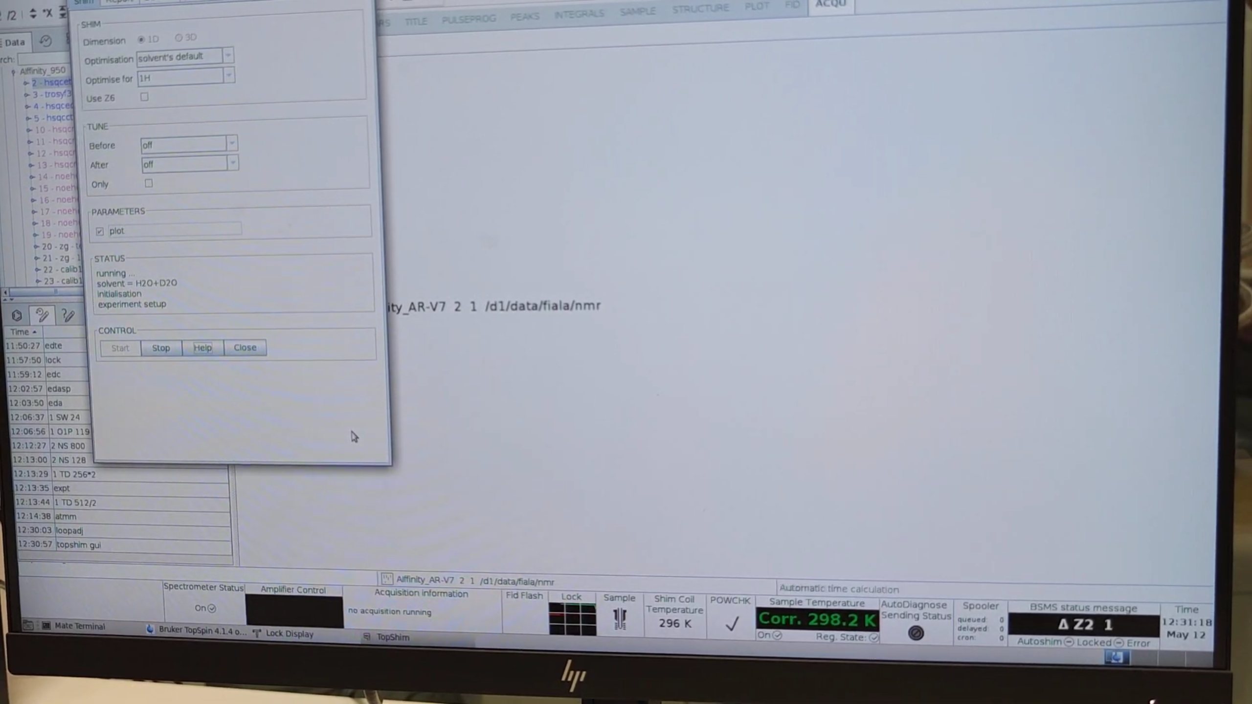
1. Under PARAMETERS type plot and start an initial shim.
2. Examine the field profile:
   • TopshimData → 1D_maps_field → zg30 (see liquid range).

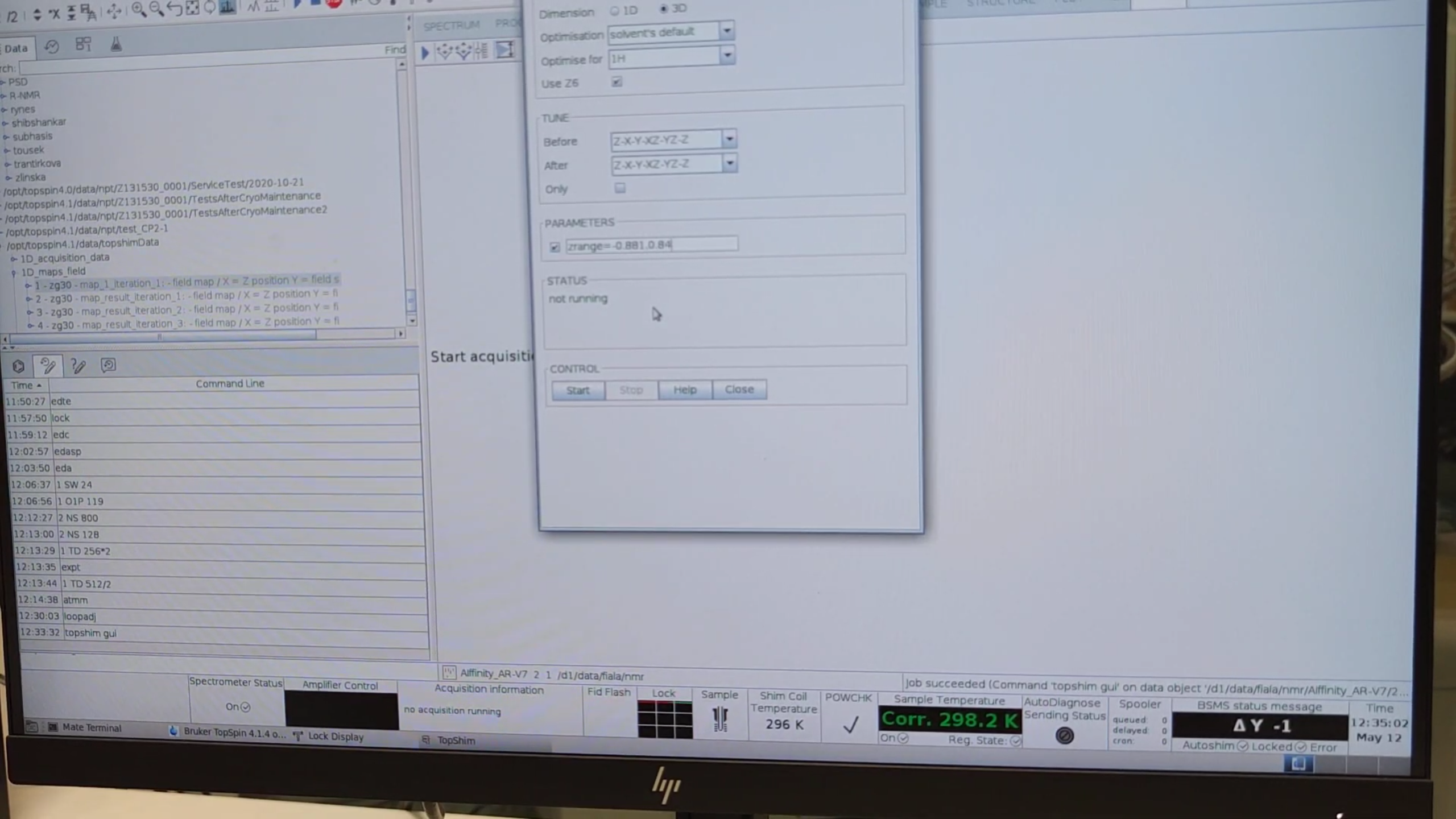
1. Run a 3D shim:
   • topshim gui → choose 3D, enable Use Z6.
   • Set Before / After to Z-X-Y-XZ-YZ-Z.
   • Under PARAMETERS enter the z-range you measured, e.g. zrange=-0.881,0.84, then click Start.

---

5. Fine-Tuning the ¹H Pulse Length

The following commands were issued in the console (no screenshots):

lockdisp
loopadj
wsh
bsmsdisp
re 1          # recall the 1D proton dataset
eda
1 AQ 0.524    # extend acquisition time
1 TD 64K
pulsecalc
ased
1 P1 1
zg            # acquire 1D ¹H
gm
ft
mc
pp

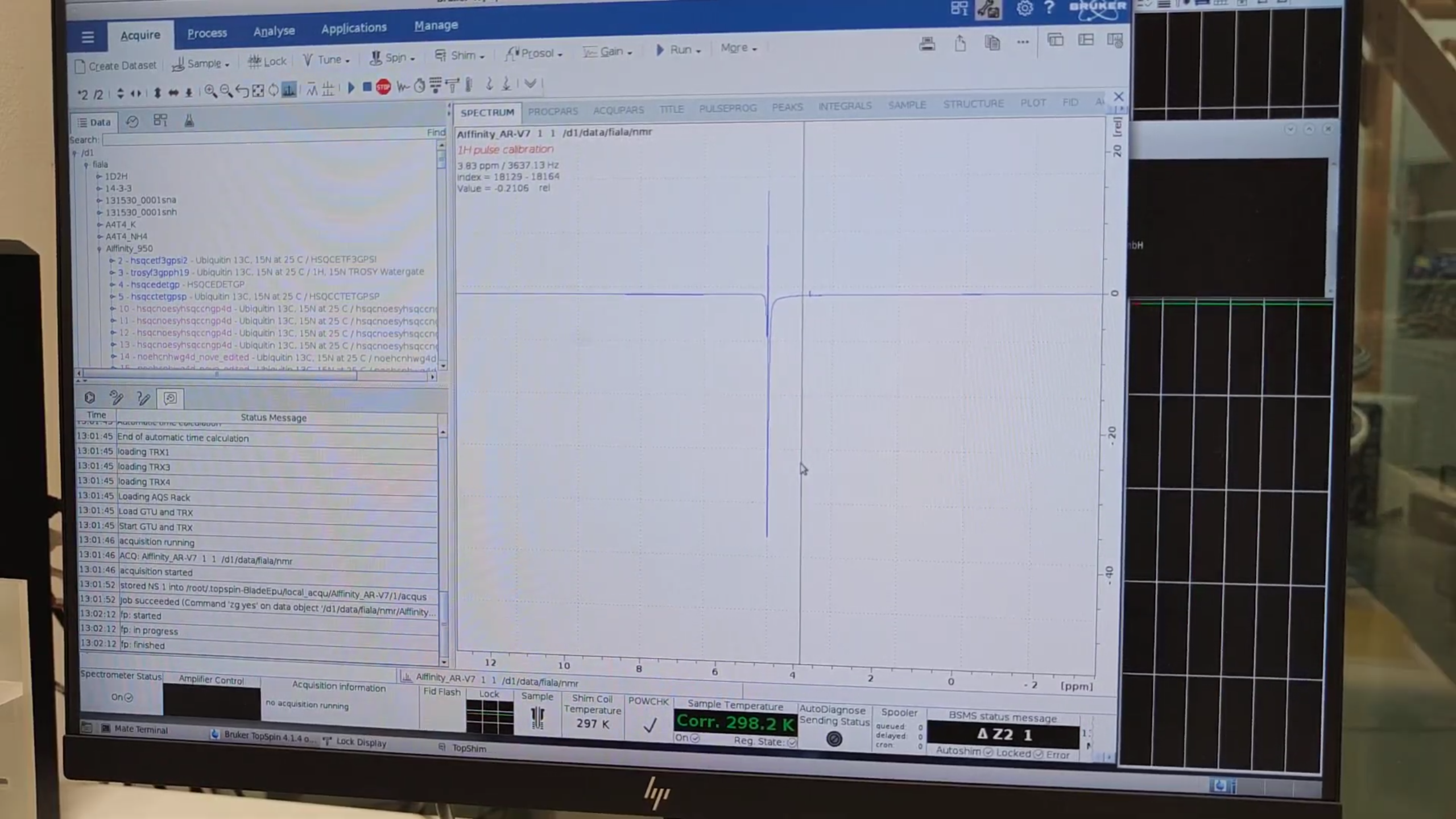
Calibrate P1

1. Open ased, set 1 P1 15.59*4.
2. Acquire (zg) the 1D proton spectrum.
3. fp → Check phasing; if lock drifted (DMSO present), re-lock.
4. .ph → manual phase → save.

5. Repeat zg to iterate pulse calibration:

   • Goal: equal positive and negative components (ideally zero net signal).
   • If more negative, increase P1 via ased (1 P1 62.520) and re-run zg.
   • Continue until balanced.

1. Divide the final P1 by 4 (90° pulse) in eda.

---

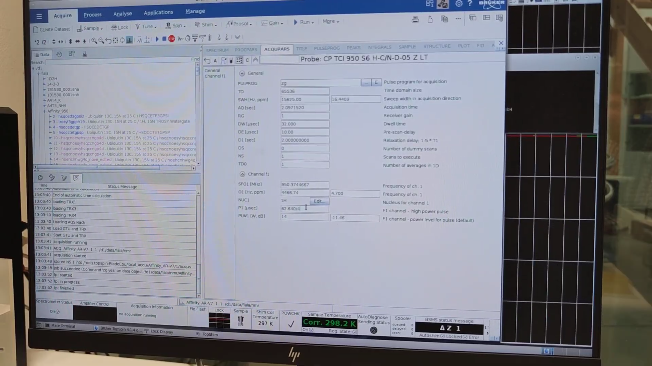
6. Water Referencing & Final HSQC Setup

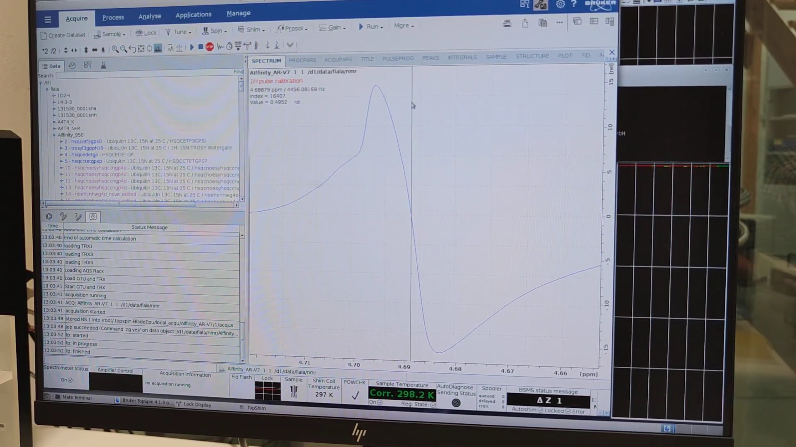
1. Zoom into the water peak, note the zero-intensity carrier (e.g. 4456.08 Hz).

2. re 2 → return to HSQC dataset → eda → set O1{F2} to that value.

3. Execute getprosol 1H 15.66 14W (15.66 µs length of 90 degree pulse, PLW1{F2}=14 W power).

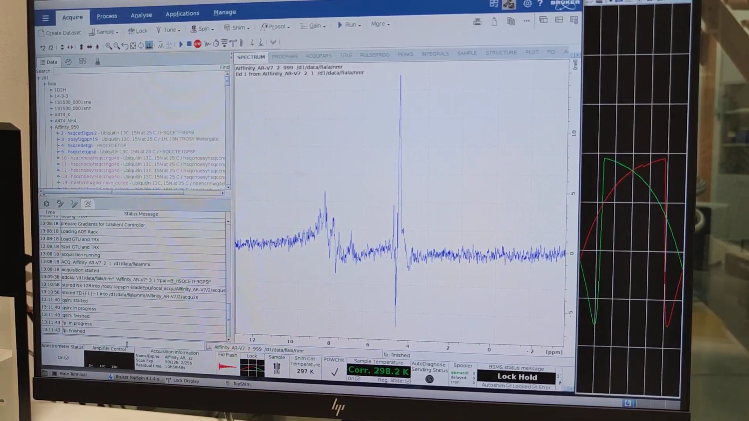
4. Verify in ased, then start the 2D HSQC: zg.

5. While acquiring, extract the 1D strip:

   • qsin → OK → peaks between 8–10 ppm confirm protein visibility.
   • Phase with .ph if needed.

---

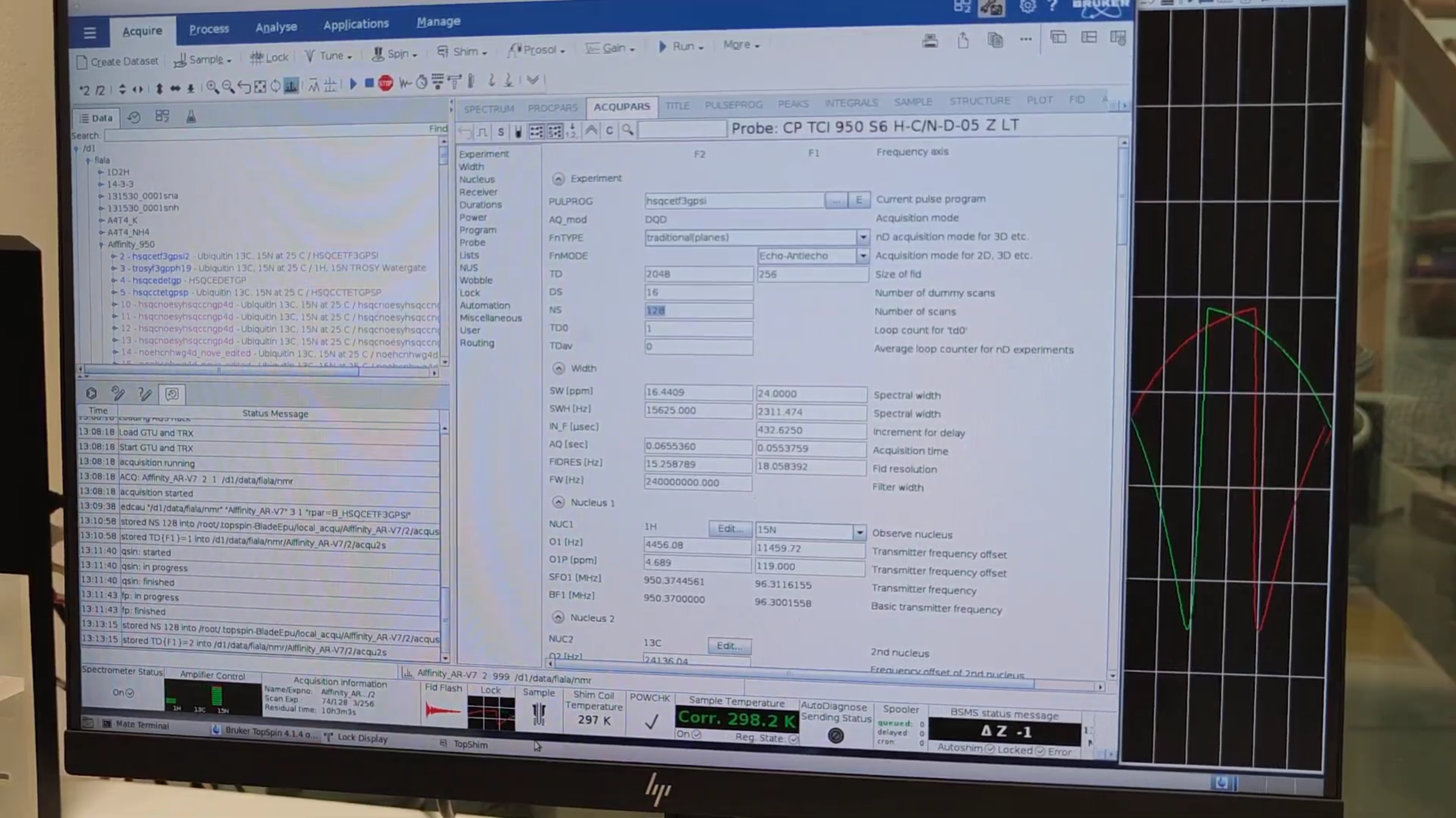
7. Setting Up the BEST-HSQC

1. Press new → Read parameters → select B_HSQCETF3GPSI (BEST variant).

2. In eda, note the shorter TD{F1} (faster but lower resolution).

   • Adjust TD, SW, NS to balance time vs. resolution.

---

8. Measuring 2D Signal-to-Noise (Classic vs. BEST)

1. Display both processed datasets side-by-side.
2. xfb → Fourier transform → abs2 then abs1 for baseline correction.
3. Synchronize views, pick a strong peak, record its region.

4. Create an int2drng file (peak1.txt) with:

   0 0
   a 2048 0 0 122.75 123.75
     16384 0 0 9.5 8.5
   a 1024 0 0 128.0 110.0
     16384 0 0 13.0 10.4
   

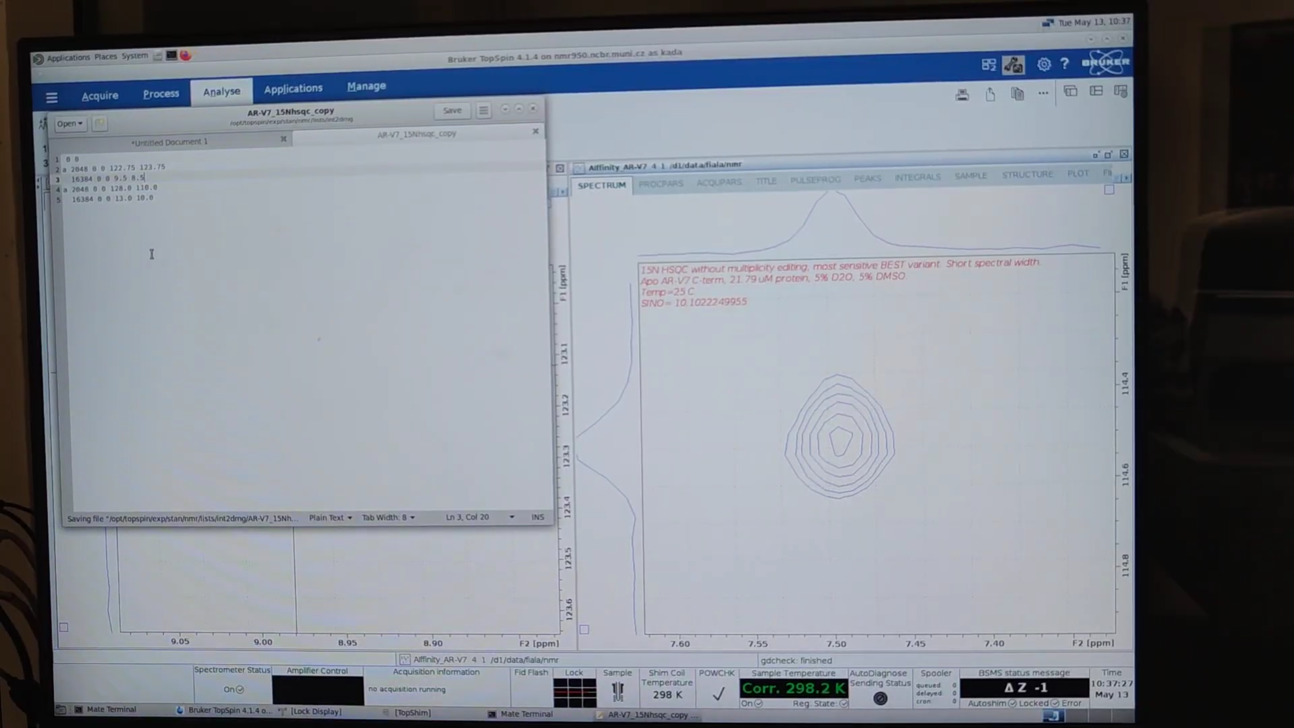
1. Run sino2D, choose peak1.txt—note SINO value.
2. Repeat for the other dataset and for 2–3 additional peaks to compare classic vs. BEST performance.

---

9. Summary Checklist

Step	Command	Purpose
New dataset	new	Copy parameters
Temperature	edte	Set temp
Parameter check	edasp, eda	Verify & edit settings
Probe tune/match	atmm	¹H & ¹⁵N matching
Lock optimize	loopadj	Fine lock
Shim	topshim gui	1-D then 3-D shim
Pulse calibration	zg, ased	Optimize P1
Water reference	eda	Set O1{F2}
Acquire HSQC	zg	Start 2D run
BEST HSQC	new → BEST sequence	Faster variant
S/N analysis	sino2D	Compare datasets

---

Authors

• Thomas Evangelidis