Tutorial on 2D Protein Spectra Processing

---

Phase Correction

• We don’t need to phase N and C dimensions.
• Before starting processing, make a copy of your 2D with wrpa, zoom into a small area of overlapping peaks, open the original 2D in another window next to the replica, click on the “exactzoom” icon, and set the same window dimensions in both spectra.
• Increase the SI size of the direct dimension up to twice the next power of 2 to increase resolution. The rest can be increased up to four times (zero filling). For example, if 15N is 256, it can be increased to 1024.
• Use xfb for the changes to take effect. The peaks should look more rounded.
• For further resolution, increase the SSB of the direct dimension to a value >2.0 (e.g. try 2.2, 2.5, 3.0).
• Use xfb again for the changes to take effect.

---

Baseline Correction and Tidying Up the Spectrum

1. Initial Setup
   • Open your spectrum in TopSpin and access the processing parameters window:
     • Click PROCPARS or type edp.
     • Ensure proper calibration for the F1 and F2 axes (SR [Hz]), paying attention to the nucleus type when referencing the calibration from 1D experiments.

2. Performing Baseline Correction

   #### Baseline Correction Overview There are two polynomial functions for baseline correction:

   1. BC_mod: Multiplies the FID (time domain) at the very beginning before the FT (takes effect after xfb).
   2. abs: Used for baseline correction on the processed spectrum (ABSG, ABSF1, ABSF2).

   #### Steps: - Set the left ABSF1 and right ABSF2 limit in the direct dimension (F2). For 15N HSQC, cover the left side of the spectrum before the water line (~4.5 ppm) to avoid noise. In general, for 15N HSQC, ABSF2 should be ≥ 5.0. - In the indirect dimension, the default values for ABSF1 and ABSF2 are typically sufficient. - Select the qpol function for baseline correction. Avoid using qfil, as it aggressively suppresses water, which may not be suitable for 15N HSQC spectra. - The 13C dimension is sensitive to the BC_mod polynomial, so avoid applying this function in such cases. - Perform FT using xfb, followed by abs1 and abs2 for baseline correction to achieve sharper and better-resolved peaks due to zero filling and increased sideband suppression (SSB).

   #### Automatic Baseline Correction for 2D Spectra: - abs2: Applies automatic baseline correction along the F2 axis. - abs1: Applies automatic baseline correction along the F1 axis. - Do first abs2 and then abs1.

3. Special Cases for Baseline Correction
   • For NOESY/ROESY Spectra (which tend to have baseline offsets, especially in t1 due to noise):
     • Use abs1 to correct the F1 direction.
     • Use abs2 to correct the F2 direction.
     • Apply t1-noise subtraction before baseline correction using the AU program t1noisereduction, which sets the lowest intensity peaks in each column of the 2D spectrum to zero. This ensures that only real peaks are displayed and reduces noise.
4. Fine-Tuning and Tidying the Spectrum
   • Water Suppression:
     • For samples in water, ONLY IF YOU HAVE NOT TRUNCATED the part of the proton dimension containing the water resonance line at ~4.7 ppm, use abs2.water for baseline correction. You can also set BC_mod=qfil in F2 to suppress the central noise stripe.

• Contour Level Adjustment:
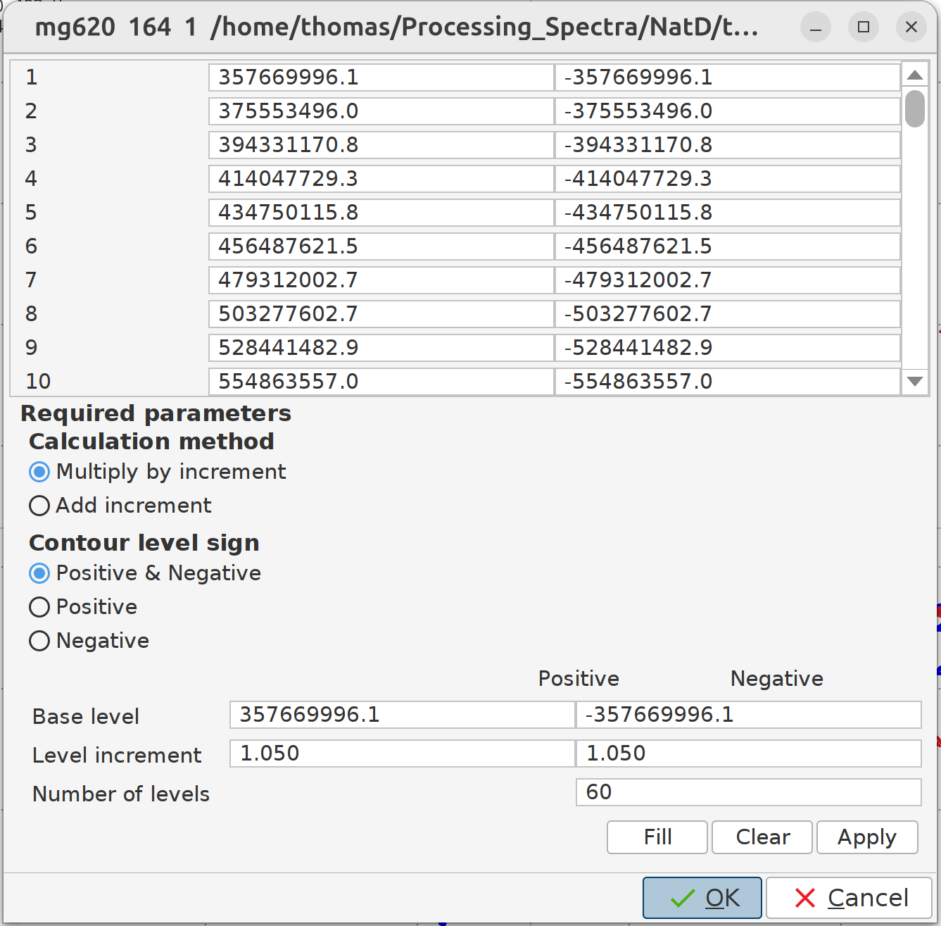
  • Manually fine-tune contour levels with the mouse button or by setting nlev to the desired number of levels. Afterward, run levcalc or clev to calculate or clear contour levels, or use edlev for manual adjustment.

    Explanation of the contour levels: The “Calculation method” defines how the “Level increment” will be applied to create the specified number of levels for both positive and negative peaks. The default is to multiply by the specified “Level increment”. You don’t need to change the “Base level” from the GUI; you can better do it with the mouse wheel by scrolling down or up. What you can change to make the peaks look more solid is to set the “Level increment”, for example, to 1.05 for both the “Positive” and “Negative”, and the “Number of levels” to 60. Then click on “Clear”, after that on “Fill”, and then on “Apply”.

1. Symmetrization (for COSY, NOESY, and ROESY Experiments)
   • After noise reduction and baseline correction, symmetrization can be applied to tidy the spectrum:
     • sym: Used for COSY spectra.
     • syma: Used for phase-sensitive experiments like NOESY. However, apply this with caution, as it can create false peaks where noise bands correlate.
2. Reducing t1-Noise
   • t1noisereduction: This program can significantly improve the tidiness of your spectra by removing low-intensity noise from the t1 dimension.
   • For t2 noise reduction swap the t1 and t2 axes with swapf1f2, followed by t1noisereduction and swapf1f2 to swap the axes back.

Linear Prediction

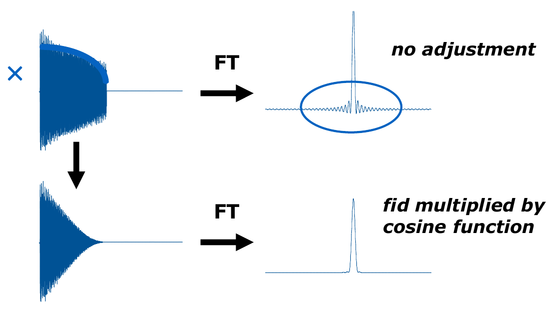
• Truncation artifacts of the FID decay can be reduced by using window functions that force the end of FID to zero.

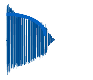
• NUS and LP should not be combined. NUS simulates fitfully the whole FID (see image below), while LP simulates the FID decay that was truncated out. As such, NUS reconstruction substitutes LP and LP must not be applied to any spectrum (4D, 3D) recorded with NUS.

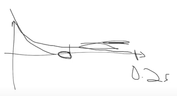
• LP is recommended only for the 15N and 13C dimensions without NUS, not for 1H dimensions (F2), because the 1H signal stops at the marked point and only noise is recorded from then on. The remaining part can be truncated to improve S/N.

• You can play with NCOEF, e.g., increase it from 32 to 48 in the indirect dimension and then use xfb.

Note

1D 1H is essential for quality control. It helps determine whether the sample is clean, detect admixtures, and monitor the water signal. It can also detect false alarms from glycerol, histidine, or other sources, and identify degradation in the 2D.

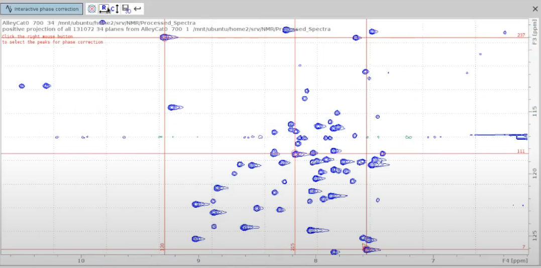
Phase Correction

• Use .ph to enter phase correction mode.
• Select two peaks from one edge of the 2D spectrum and one from the opposite edge, as well as at least one in the intermediate region. It is important to cover the whole spectrum to monitor the effect of phase correction on distant peaks.

---

Authors

• Thomas Evangelidis