NUS Reconstruction of 4D spectra in Topspin
Table of contents
- General workflow
- Examples
- Bruker 4D HCNH NOESY
hsqcnoesyhsqccngp4d -
[AI ffinity custom 4D HMQC-NOESY-HSQC experiment noehcnhwg4d_nove](#aiffinity-custom-4d-hmqc-noesy-hsqc-experiment-noehcnhwg4d_nove) - Frank Lohr’s implementation of 4D HMQC-NOESY-HSQC experiment
sfhmqc_noe_sfhmqc_4Dhcnh.fl
- Bruker 4D HCNH NOESY
- Credits
Tested environment:
- Topspin 4.4.0 with commercial license for NUS processing
- OS: AlmaLinux 9 (as an Oracle virtual machine)
- 20 CPU cores, 120 GB of RAM.
Caution Not everything is thoroughly tested yet
General workflow
- Copy the raw 4D spectrum in a new directory by executing
wrpacommand. This will make working with the 4D neat and safe.
Note: NUS FIDs before reconstruction are not that heavy: the
serfiles are usually <1 Gb.
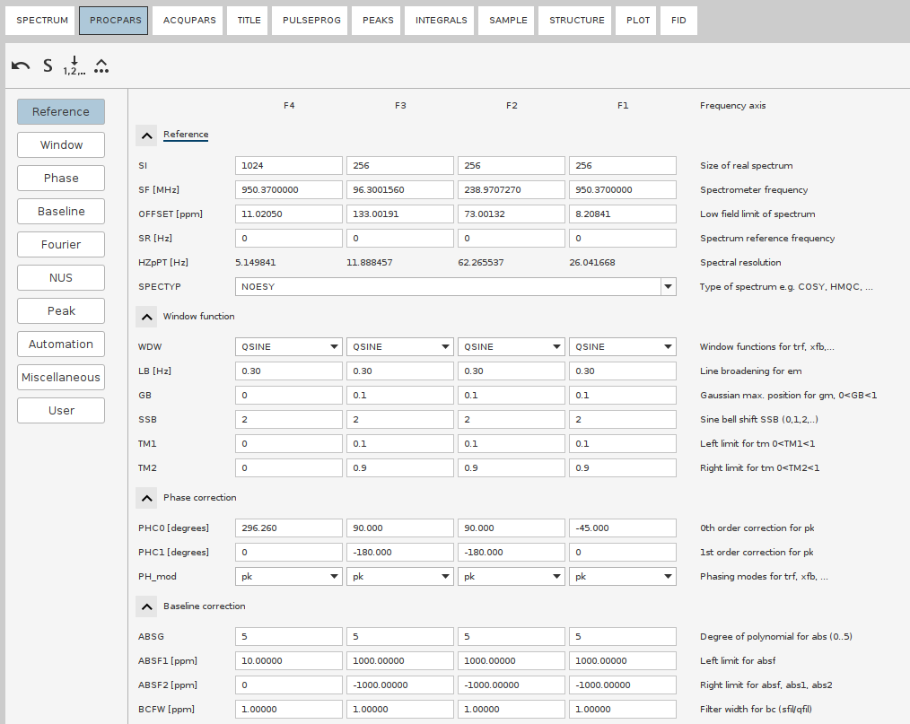
- Switch to the newly copied procedure; Open up the processing parameters (
edpor the tabPROCPAR). - Adjust the size of the dimensions in the final spectrum with the parameter
SI. Always set it to a power of 2. For example, ifTDvalues underACQUPARSis160, then seSIto256or512.
Important: Always set the
SIto the next or higher power of 2, never lower than the respectiveTDvalue! Otherwise TopSpin behaves weirdly, e.g. will leave indirect dimensions in time domain.
- If there were recorded test 2D planes (or 3D cubes) with this exact 4D pulse program, check their processing parameters:
- Phasing in the direct and indirect dimensions
- Window functions (rarely changes from default)
- Baseline correction parameters (rarely changes from default)
- Linear Prediction (LP), if you use it.
Tip: NUS and LP should not be combined. NUS simulates fitfully the whole FID, while LP simulates the FID decay that was truncated out. As such, NUS reconstruction substitutes LP and LP must not be applied to any spectrum (4D, 3D) recorded with NUS. If recorderd without NUS, Using LP can enhance resolution, especially if the time domain (TD) values are small or if your FIDs are truncated. In TopSpin, you can use LP for improving resolution in particular dimensions during the Fourier Transform process by specifying the
ME_modandNCOEFparameters for those dimensions. Note that it may cause additional wiggles.
- The NUS parameters must be set according to the
PHC0andPHC1Phase angles of the indirect dimensions.- Set the
MddPHASE{Fi}parameter to the same value as thePHC0{Fi}. - For any indirect dimension i with
PHC1{Fi} == 180, set theMddF180{F1}parameter to TRUE.
- Set the
- Set the
FnMODEaccording to the acquisition mode (usually theNdimension isecho-antiechoand the restStates-TPPI) - Note down the signal region in the direct dimension. It can be extracted either from the test planes or the 2D experiments (HSQC, TOCSY, etc).
- Go to the 2D experiment. Zoom in such that the signal-free regions are trimmed as much as possible. Issue the
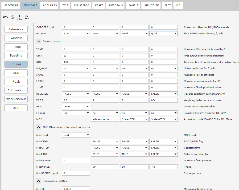
.ftf2region STSRcommand, it will prompt toSave display region to Parameters STSR\SI. - Issue the
STSRcommand. Note down the values for the direct dimension. Same withSTSI
- Go to the 2D experiment. Zoom in such that the signal-free regions are trimmed as much as possible. Issue the
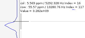
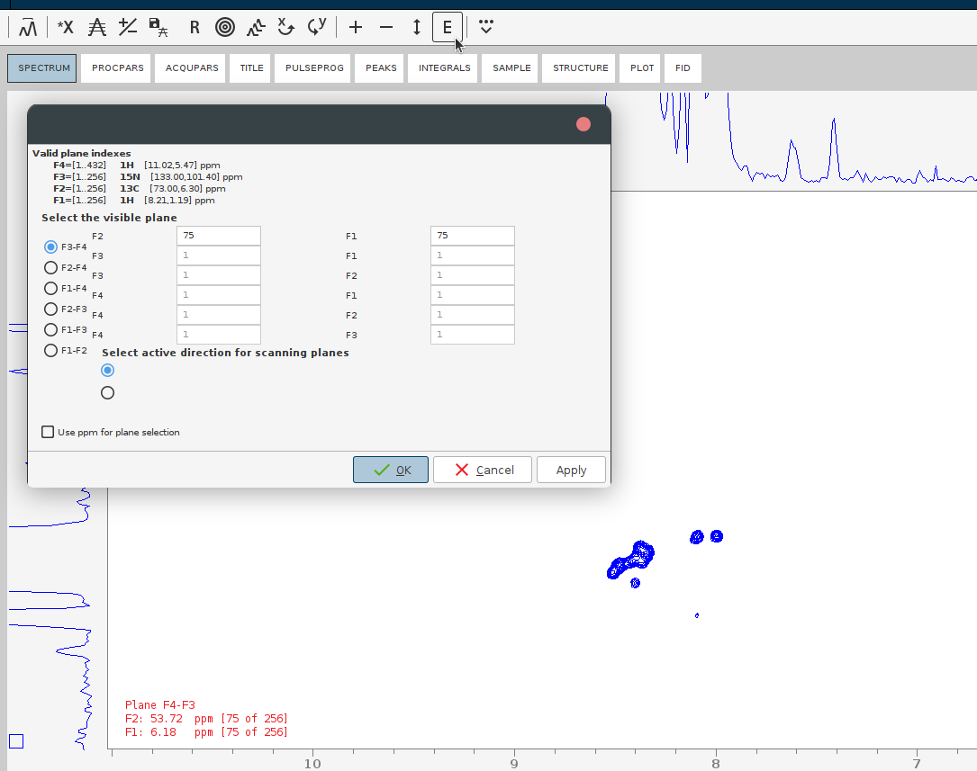
Tip: Those values may be obtained manually: in the 1D or 2D spectrum, note the “col Index” (
16on the screenshot). Save it intoSTSR. Move the coursor to the right and calculate the width of the dimension in points, save that number intoSTSI.
Important: If you copy the FT region from the planes, make sure the spectrum windows (SW) of the 4D and the test planes are the same. If they are not, the signal regions have to be adjusted manually.
- Go to the
NUSsection. Set the NUS mode tocs. Set the phasing of the indirect dimensions to the same values as in thePhasesection (i.e.PH0andPH1). - For the CS reconstructions in Topspin, it’s a good idea to increase the number of iterations. Since 4D spectra have
a high dynamic range, weaker peaks are typically reconstructed in later iterations. The default setting of
Mdd_CsNITER 200(hidden parameter) in Topspin could be increased toMdd_CsNITER 400orMdd_CsNITER 600for better results. However, this should be tested case by case. While you may be tempted to go up to 1000 iterations, this is likely unnecessary. -
When everything is ready, issue
ftnd 0 nusthreads 16
ftndwill run the NUS reconstruction, followed by FT all directions, with the Window Multiplication (WM) and baseline correction as specified in the PROCPARS.0stands for “all dimensions”,nusthreads 16allocates 16 CPU cores for the process (Topspin’s limit).
Note: Whereas NUS reconstruction is parallelized, FT stage uses only a single thread, therefore takes multiple hours.
- Optionally: adjust baseline correction parameters and apply the automatic baseline correction to the whole reconstructed 4D spectrum.
- I am not sure whether baseline correction only in F4 or in all F1-F4 would be better - if better than without baseline correction.
Topspin offers the command
absndbut you have to execute it for each dimension individually, which is tedious as the processing of each dimension lasts long. To run it on all 4 dimensions automatically we will create a new macro. edmacto create a new macro and then File -> New. Name the new macroabs4dand in the window that will pop up write:absnd 4 absnd 3 absnd 2 absnd 1- issue the macro command
abs4dto launch the baseline correction in the order F4, F3, F2, F1.
- I am not sure whether baseline correction only in F4 or in all F1-F4 would be better - if better than without baseline correction.
Topspin offers the command
- Evaluate the quality of the reconstructed spectrum by looking at the sum projections. You need to look at both positive and negative projections to identify the antiphase signals as well as the potentially misphased peaks. This is done by the command
projplpandprojpln. Run each and provide the parameters over the GUI or run the single lines such asprojplp 12 all all 21projplpstands for positive projection; runprojplnto get the negative one12refers to keeping the first two dimensions (for standard Bruker HSQC NOESY, those are C and HC dimensions); that means, N (F3) and direct H (F4) will be summed up.allindicates that all planes within these dimensions should be included.21specifies the output PROCNO where the projection data will be stored. Adjust the PROCNO based on where you want to save the output.
- Perform automatic baseline correction of the projections with
abs1followed byabs2. - If the projections look good, evaluate the 4D spectrum.
- Perform a putative peak picking. For that, lower the countours such that the noise disappears, then issue
ppand set the sensitivity to the lowest countour level.
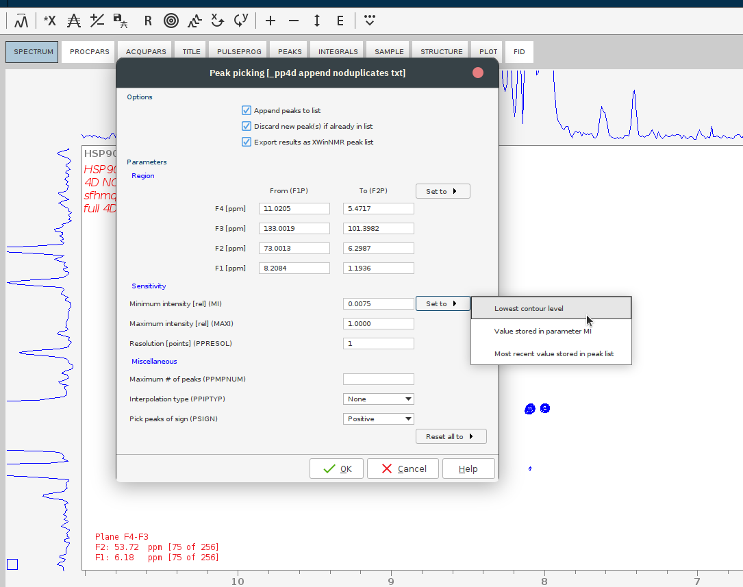
- Jump to some position of the 4D which contains signals. For that, press the E button and give the plane numbers or the desired ppm.
- Perform a putative peak picking. For that, lower the countours such that the noise disappears, then issue
- If the phasing or other processing parameters are off, adjust them and repeat the NUS reconstruction. If the projections look good - congratulations!
Troubleshooting
Post-reconstruction phasing
If the spectrum appears to be misphased, it has to be processed all over again. To determine the optimal phasing angles:
The reconstructed spectrum is left in the time domain
- Run
ftnd 3,ftnd 2andftnd 1to reconstruct the dimensions one by one.- This should not initiate NUS reconstruction, at least on the machines without the NUS license.
Examples
Bruker 4D HCNH NOESY hsqcnoesyhsqccngp4d
The test protein is Ubiquitin measured on the 600 MHz spectrometer.
Download the raw 4D spectrum (Topspin directory of the experiment)
Axis order:
| F4 | F3 | F2 | F1 |
|---|---|---|---|
| HN | N | Hc | C |
Processing steps
-
Set Main Processing Parameters (
edp):F4 F3 F2 F1 SI 1024 256 512 256 PHC0 150 0 0 0 PHC1 0 0 0 0 PH mod pk pk pk pk BC_mod qfil or qpol no no no STSR 55 0 0 0 SRSI 350 0 0 0 FCOR 0.5 0.5 0.5 0.5 NUS Mdd_mod cs MddF180 false false false MdPHASE 0 0 0
Linear Prediction in the F1 (C) and F3 (N) dimensions is not recommended with this PP. In my experience it introduces noise.
Optionally increase the number of iterations with Mdd_CsNITER 600.
The following parameters are automatically set:
- MDD_CsAlg:
IST - MDD_CsVE:
true
-
Process 4D Spectrum:
ftnd 0 -
Optional Baseline Correction in F4:
absnd 4 - Correct shift of HC(F2) axis:
- In Topspin: set
SR(F2) to (11.9037/4)*600.05=1785.70 Hz - In POKY: set HC shift in
stto -(11.9037/4)=-2.976 ppm
- In Topspin: set
- Pick the most intense peaks with
ppinterface - Make the projections:
projplp 34 all all 43projpln 34 all all 430projplp 24 all all 42projpln 24 all all 420projplp 14 all all 41projpln 14 all all 410projplp 23 all all 32projpln 23 all all 320projplp 13 all all 31projpln 13 all all 310projplp 12 all all 21projpln 12 all all 210
- Evaluate the projections and the spectrum visually by jumping from peak to peak
AI|ffinity custom 4D HMQC-NOESY-HSQC experiment noehcnhwg4d_nove
The test protein is Ubiquitin measured on the 600 MHz spectrometer.
Download the raw 4D spectrum (Topspin directory of the experiment)
Axis order:
| F4 | F3 | F2 | F1 |
|---|---|---|---|
| HN | N | C | Hc |
Processing steps
- Correct 1-Point Delay in 13C:
- Create a new nuslist with a 1-point shift in the 13C axis and replace the original nuslist:
awk '{print $1,$2+1,$3}' nuslist > nuslist.off mv nuslist nuslist.back mv nuslist.off nuslist - Extend the 13C axis in Topspin by 1 complex point by changing static param NusTD(F2) from
160(TD(F2)in yourACQPARS) to162(TD(F2)+2):2s NusTD 162Verify that
162was saved in the file:grep "NusTD" acqu3sThis should automatically set static TDeff(F2) also to
162and allow processing with the adjusted nuslist.
- Create a new nuslist with a 1-point shift in the 13C axis and replace the original nuslist:
-
Set Main Processing Parameters (
edp):F4 F3 F2 F1 SI 1024 256 256 512 PHC0 -107 0 0 0 PHC1 0 0 0 0 PH mod pk pk pk pk BC_mod qfil or qpol no no no STSR 55 0 0 0 SRSI 350 0 0 0 FCOR 0.5 0.5 0.5 0.5 NUS Mdd_mod cs MddF180 false false false MdPHASE 0 0 0
Optionally increase the number of iterations with Mdd_CsNITER 600.
The following parameters are automatically set:
- MDD_CsAlg:
IST - MDD_CsVE:
true
-
Process 4D Spectrum:
ftnd 0 -
Optional Baseline Correction in F4:
absnd 4 - Correct Known TopSpin Bug (Badly Written CAR) + Correct Shift by 1/4*SW in 13C:**
- CAR of HC Axis: Written as 6.666 ppm, but should be 4.7 ppm
- Total shift of HC(F1) axis:
- In Topspin: Set SR(F1) to (6.666-4.7)*600.05 = 1179.698 Hz or
- In POKY: Set HC shift in “st” to -(6.666-4.7) = -1.966 ppm
- Total shift of HC(F1) axis:
- CAR of 13C Axis: Written as 39.1096 ppm, but should be 41 ppm. 13C axis is folded by 1/4*SW, relevant peaks are aliased.
- Total shift of 13C(F2) axis:
- In Topspin: Set SR(F2) to (58.0333/4 + (41-39.1096))*150.882693 = 2474.283 Hz or
- In POKY: Set 13C shift in “st” to -(58.0333/4 + (41-39.1096)) = -16.398 ppm
- Total shift of 13C(F2) axis:
- CAR of HC Axis: Written as 6.666 ppm, but should be 4.7 ppm
- Pick the most intense peaks with
ppinterface - Make the projections:
projplp 34 all all 43projpln 34 all all 430projplp 24 all all 42projpln 24 all all 420projplp 14 all all 41projpln 14 all all 410projplp 23 all all 32projpln 23 all all 320projplp 13 all all 31projpln 13 all all 310projplp 12 all all 21projpln 12 all all 210
- Evaluate the projections and the spectrum visually by jumping from peak to peak
Frank Lohr’s implementation of 4D SOFAST-HMQC-NOESY-HSQC experiment sfhmqc_noe_sfhmqc_4Dhcnh.fl
The test protein is SAK 42D (15.58 kDa) measured on the 950 MHz spectrometer.
Download the raw 4D spectrum (Topspin directory of the experiment)
Axis order:
| F4 | F3 | F2 | F1 |
|---|---|---|---|
| HN | N | C | Hc |
On the example of the Exp. 72 (Ubiquitin)
Processing steps
-
Set Main Processing Parameters (
edp):F4 F3 F2 F1 SI 1024 128 256 256 PHC0 -68 90 90 -45 PHC1 0 -180 -180 0 PH mod pk pk pk pk BC_mod no no no no STSR 0 0 0 0 SRSI 400 0 0 0 FCOR 0.5 1.0 1.0 0.5 NUS Mdd_mod cs MddF180 true true false MdPHASE 90 90 -45
Note: This specific phasing in the indirect dimension takes care of the 1-point delay incorporated into the pulse program in ¹³C channel.
Optionally increase the number of iterations with Mdd_CsNITER 600.
The following parameters are automatically set:
- MDD_CsAlg:
IST - MDD_CsVE:
true
-
Process 4D Spectrum:
ftnd 0 -
Optional Baseline Correction in F4:
absnd 4 - Correct Shift of HC(F1) Axis:
- In Topspin: Set SR(F1) to (O1P-CNST16)BF1 = (4.7-2.75)950.37 = 1853.22 Hz or
- In POKY: Set HC shift in “st” to -(O1P-CNST16) = -(4.7-2.75) = -1.95 ppm
-
Pick the most intense peaks with
ppinterface - Make the projections:
projplp 34 all all 43projpln 34 all all 430projplp 24 all all 42projpln 24 all all 420projplp 14 all all 41projpln 14 all all 410projplp 23 all all 32projpln 23 all all 320projplp 13 all all 31projpln 13 all all 310projplp 12 all all 21projpln 12 all all 210
- Evaluate the projections and the spectrum visually by jumping from peak to peak
Authors
- Petr Padrta, 14.6.2024
- Thomas Evangelidis
- Ekaterina Burakova