Protein Backbone 3D NMR Spectra Acquisition Workflow
This tutorial contains of experiments for a 14 kDa IDP conducted on 950 MHz but without 13C and 15N hard pulse calibrations. For 13C and 15N pulse calibration for the same protein on the 850 MHz refer to this tutorial.
1 · Initial Calibrations and Test HSQCs
First we did 1H pulse calibration (exp. 1), while for 13C and 15N we used the default parameters from getprosol.
Then we measured a short 15N HSQC (exp. 2) and a short 13C HSQC (exp. 3) with full spectral width on N and C, respectively.
2 · CBCAcoNH N–HN Plane Comparison
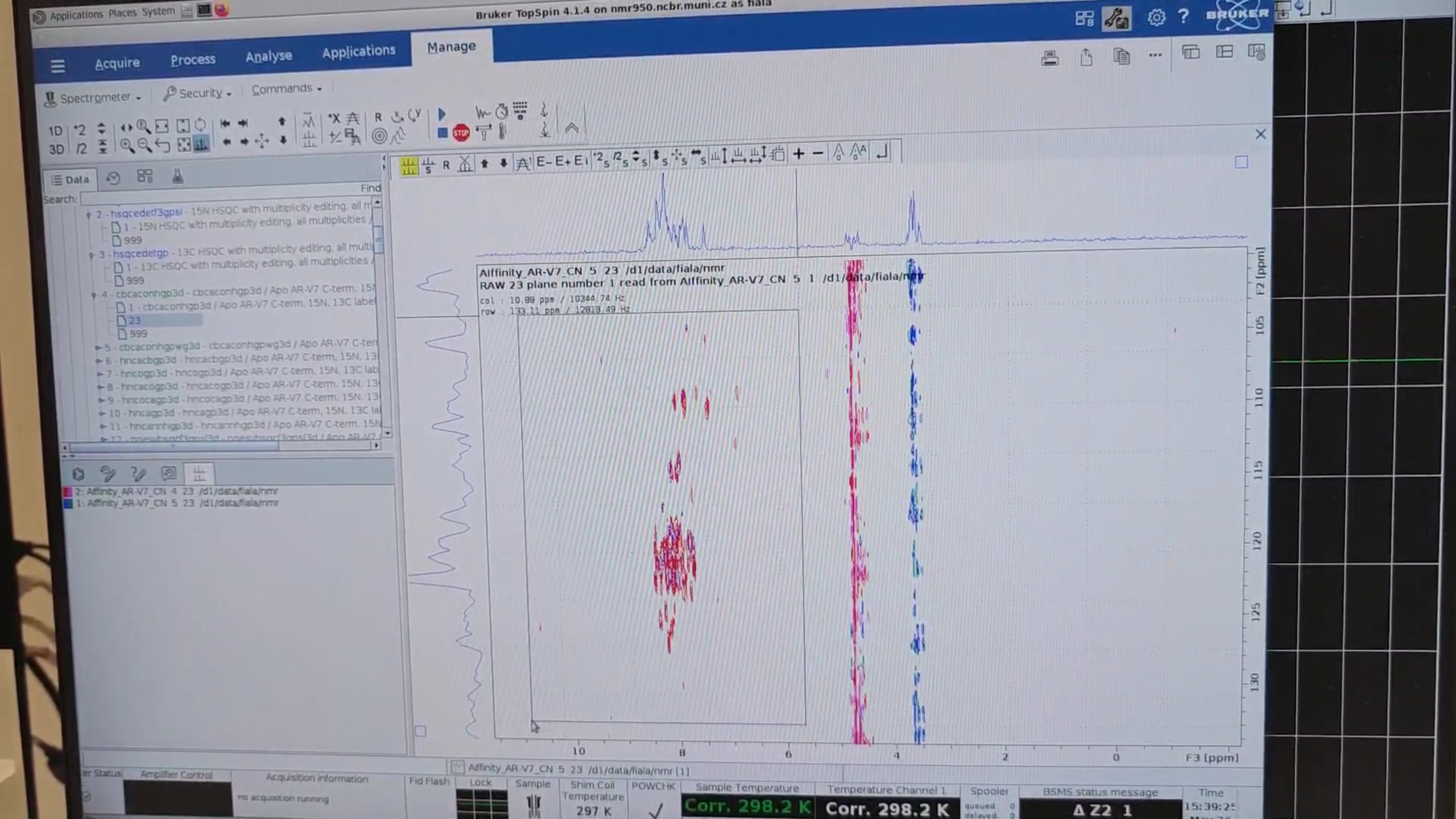
We also measured the N–HN planes of two types of CBCAcoNH pulse programs, the standard version and the one with Water-Gate, and we want to select the best one for this sample.
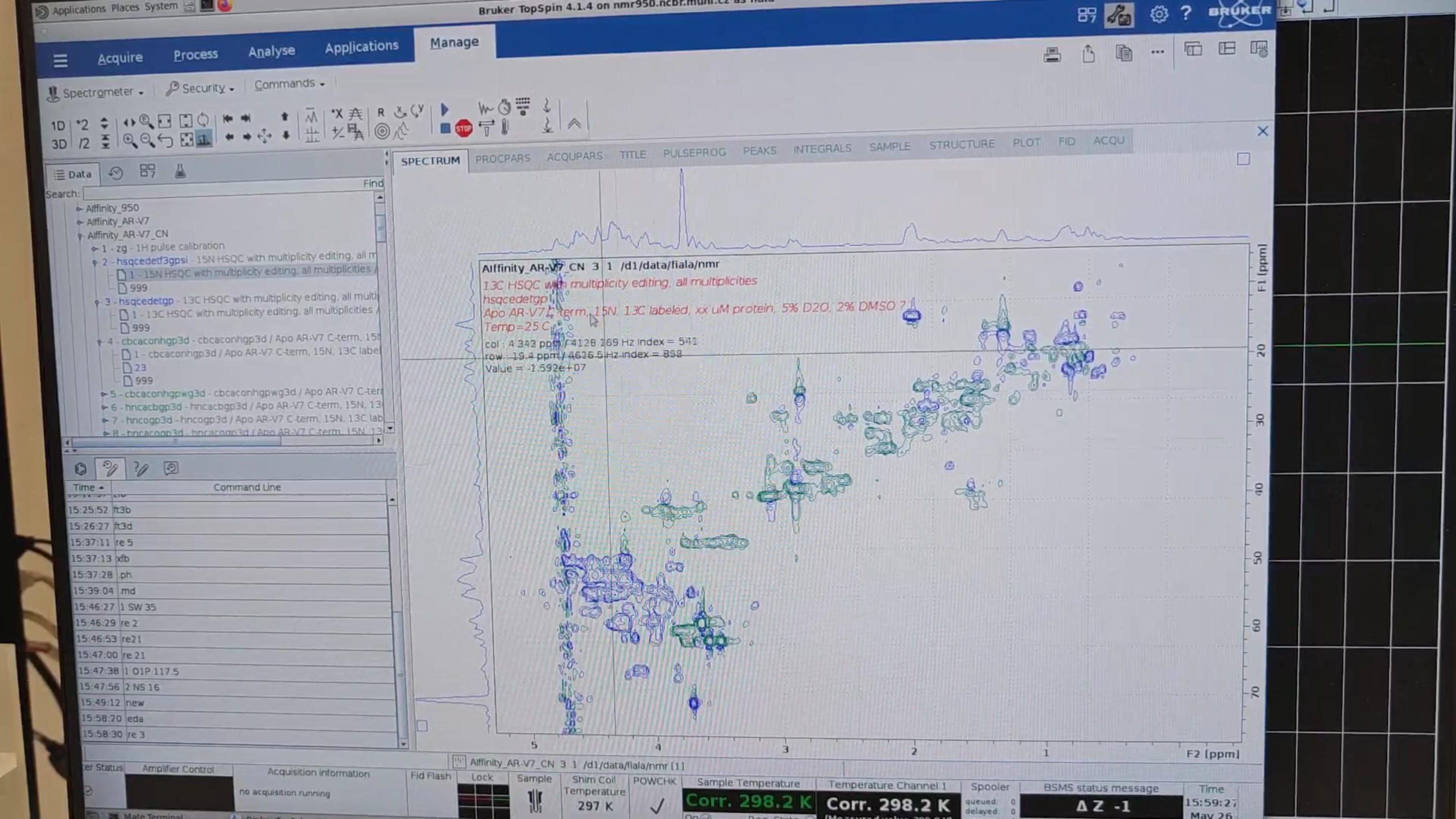
xfb– process the N–HN planes from both CBCAcoNH experiments (exp. 4 and 5) and then.phto correct their phase..md– overlay the N–HN planes from exp. 4 and 5, then click “copy the contour levels from first to other datasets.” The standard version (red; exp. 4) seems to be more sensitive.
3 · Set-Up of Full-Length HSQC Experiments
re 2 to display the test 15N HSQC (experiment 2) and hit new to create a new 15N HSQC with the desired spectral
width in the N dimension. Name it 21.
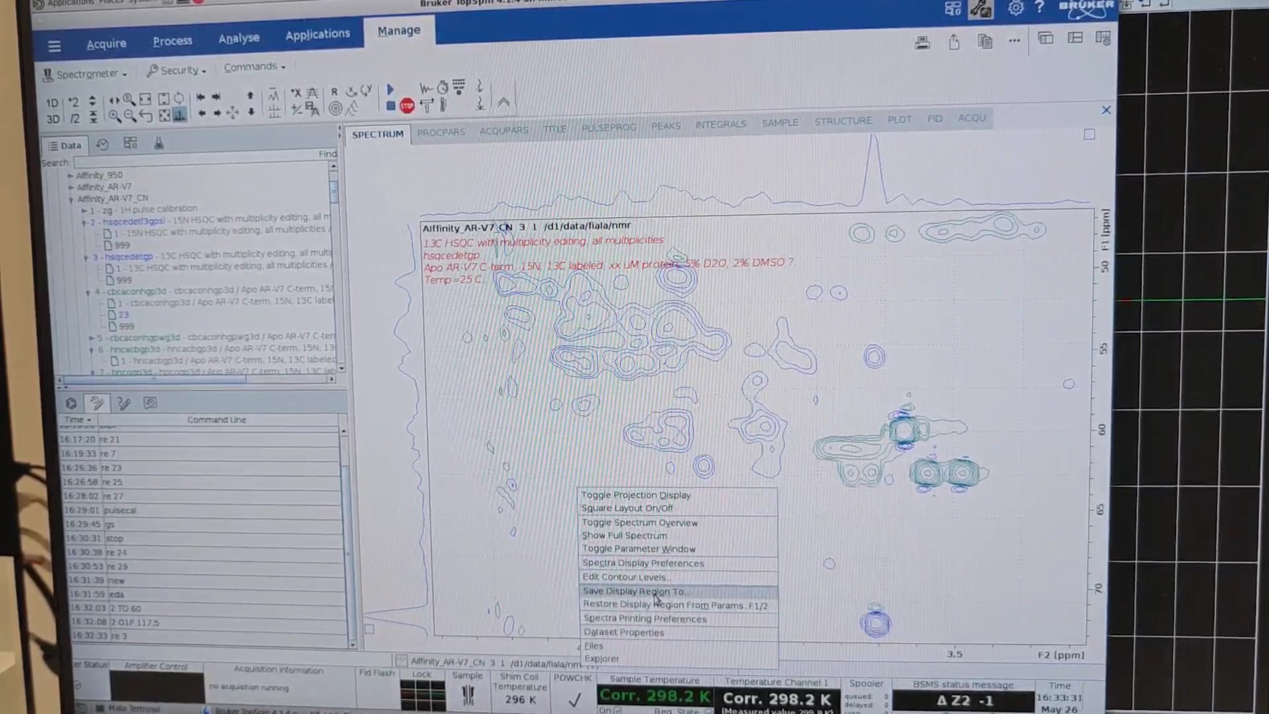
re 2 again, zoom into the region of interest, then Right-click → Save Display Region To… → Parameters ABSF1/2. In
PROCPARS note the N-axis boundaries, e.g. 100 ppm → 135 ppm.
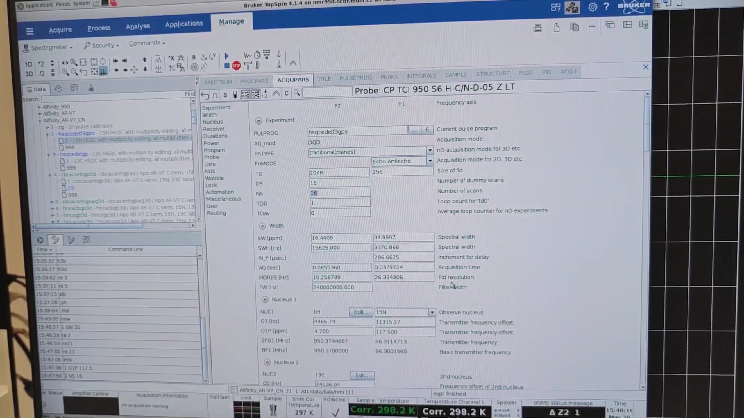
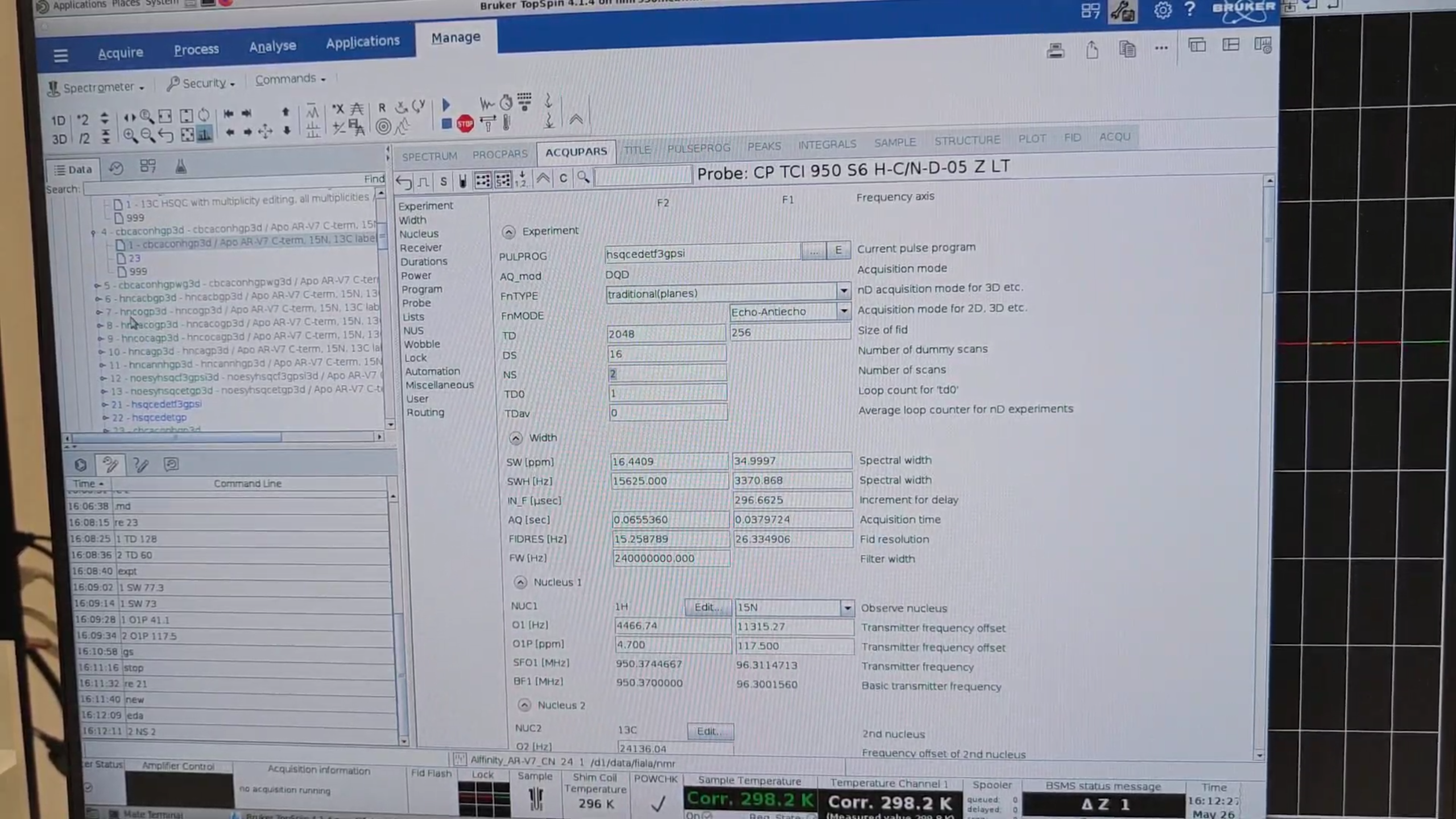
re 21, then eda to open ACQUPARS. Set:
| Parameter | Value |
|---|---|
SW{F1} |
135-100 ppm |
O1P{F1} |
100+(135-100)/2 ppm |
NS |
16 |
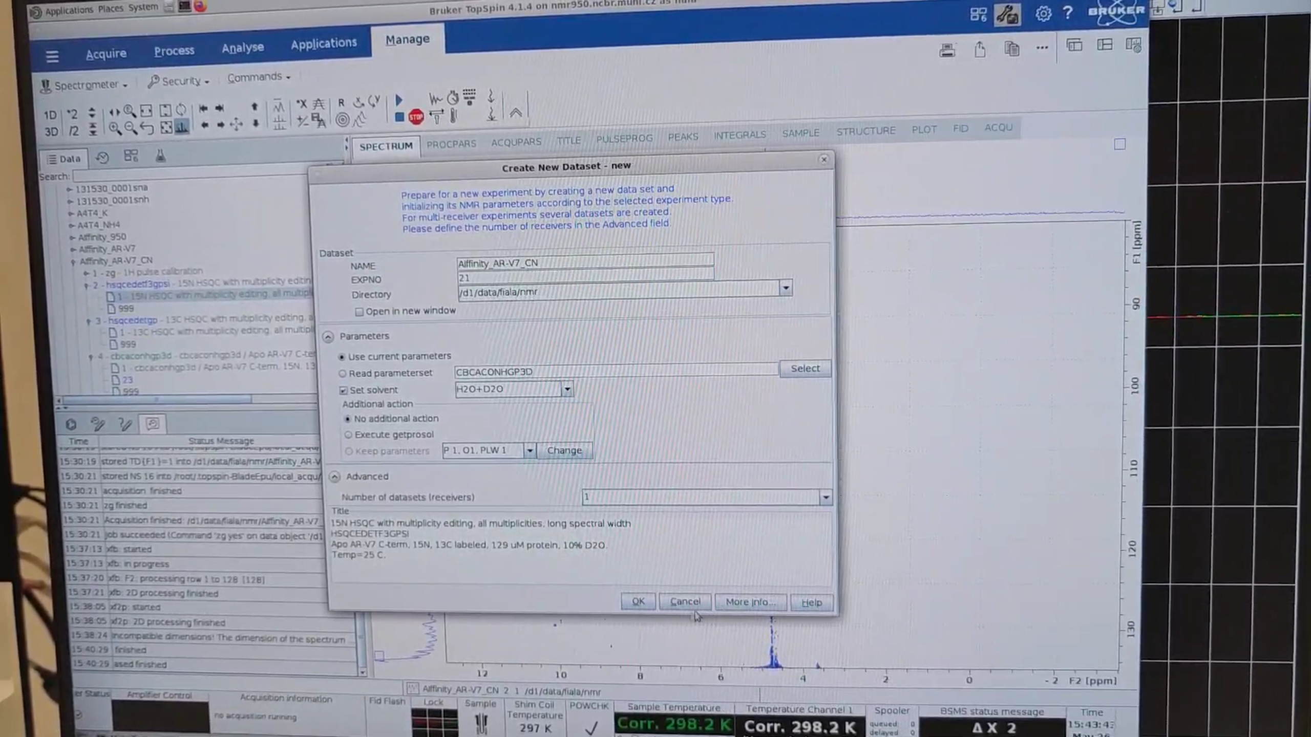
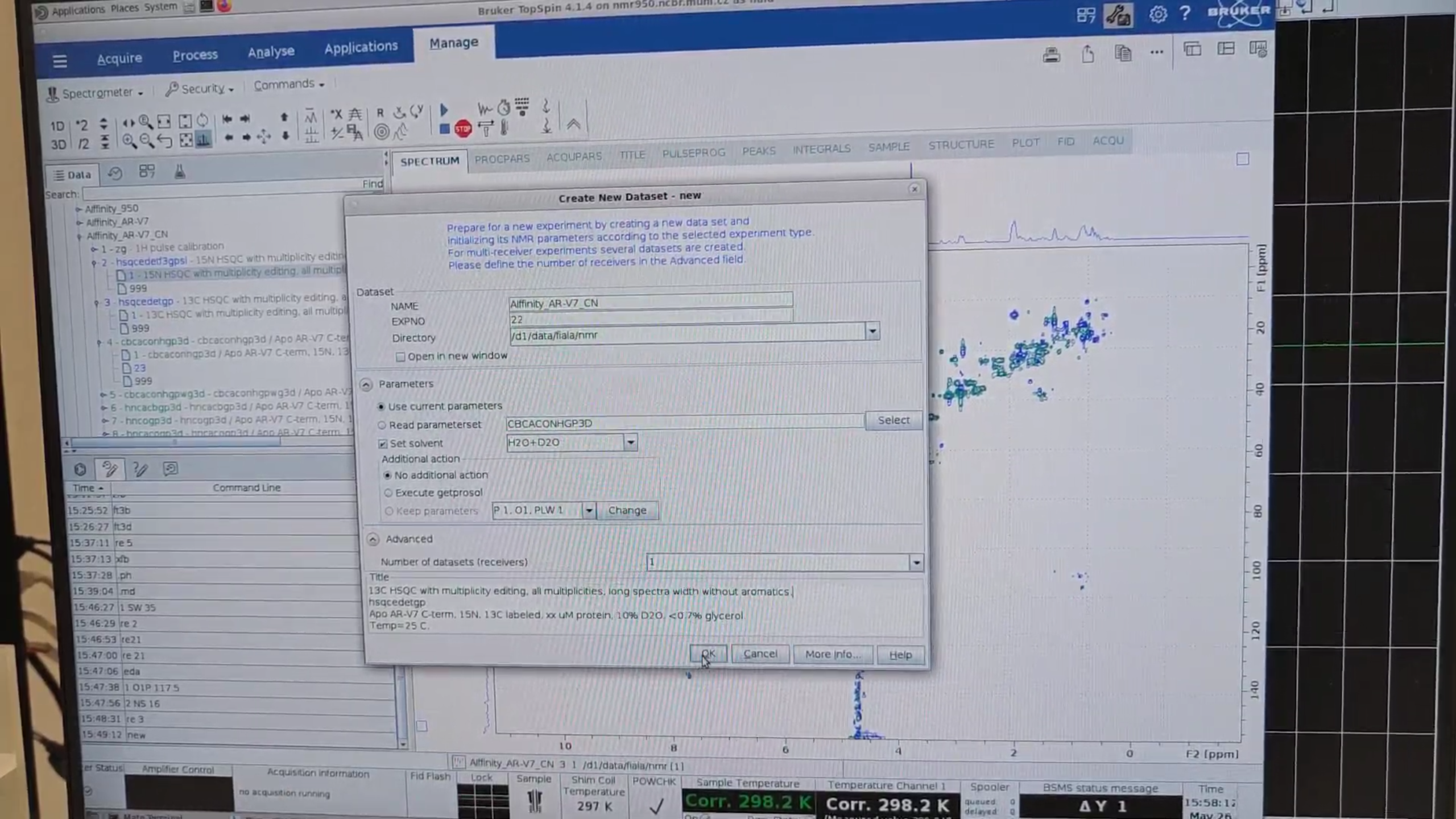
re 3, followed by new, to create a full 13C HSQC from the test 13C HSQC (experiment 3). Name it 22.
re 3 again, zoom into the region of interest, then Right-click → Save Display Region To… → Parameters ABSF1/2.
Record the aliphatic-C limits, e.g. 4.6 ppm → 77.5 ppm.
re 22, then eda and set:
| Parameter | Value |
|---|---|
SW{F1} |
77.5-4.6 (=72.9) ppm |
O1P{F1} |
4.6 + 72.9 ⁄ 2 (=41.05) ppm |
NS |
16 |
Run expt to estimate the experimental time.
4 · Set-Up of CBCAcoNH Experiments
Note the N and aliphatic-C spectral widths from the 15N HSQC (exp. 21) and 13C HSQC (exp. 22).
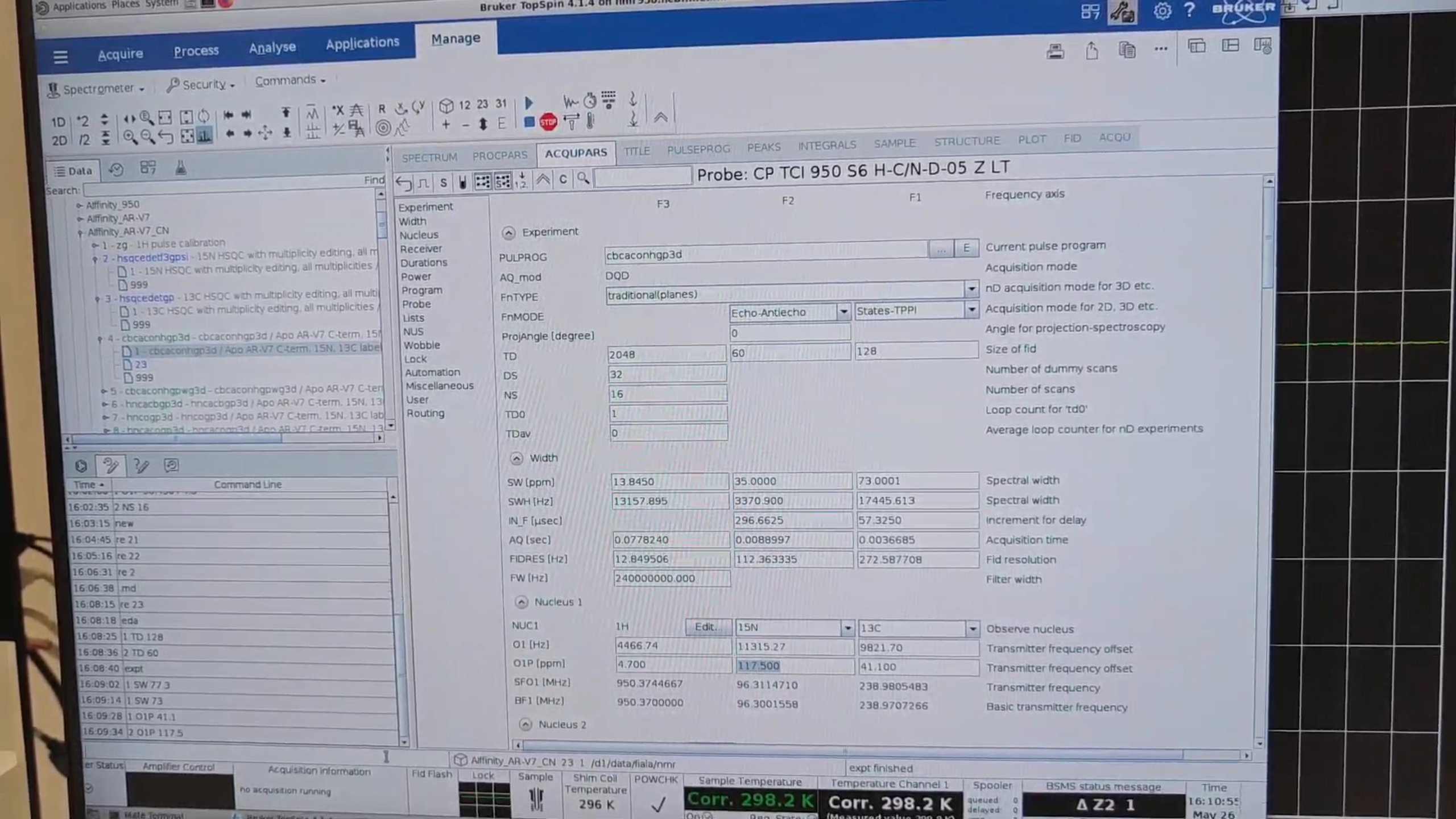
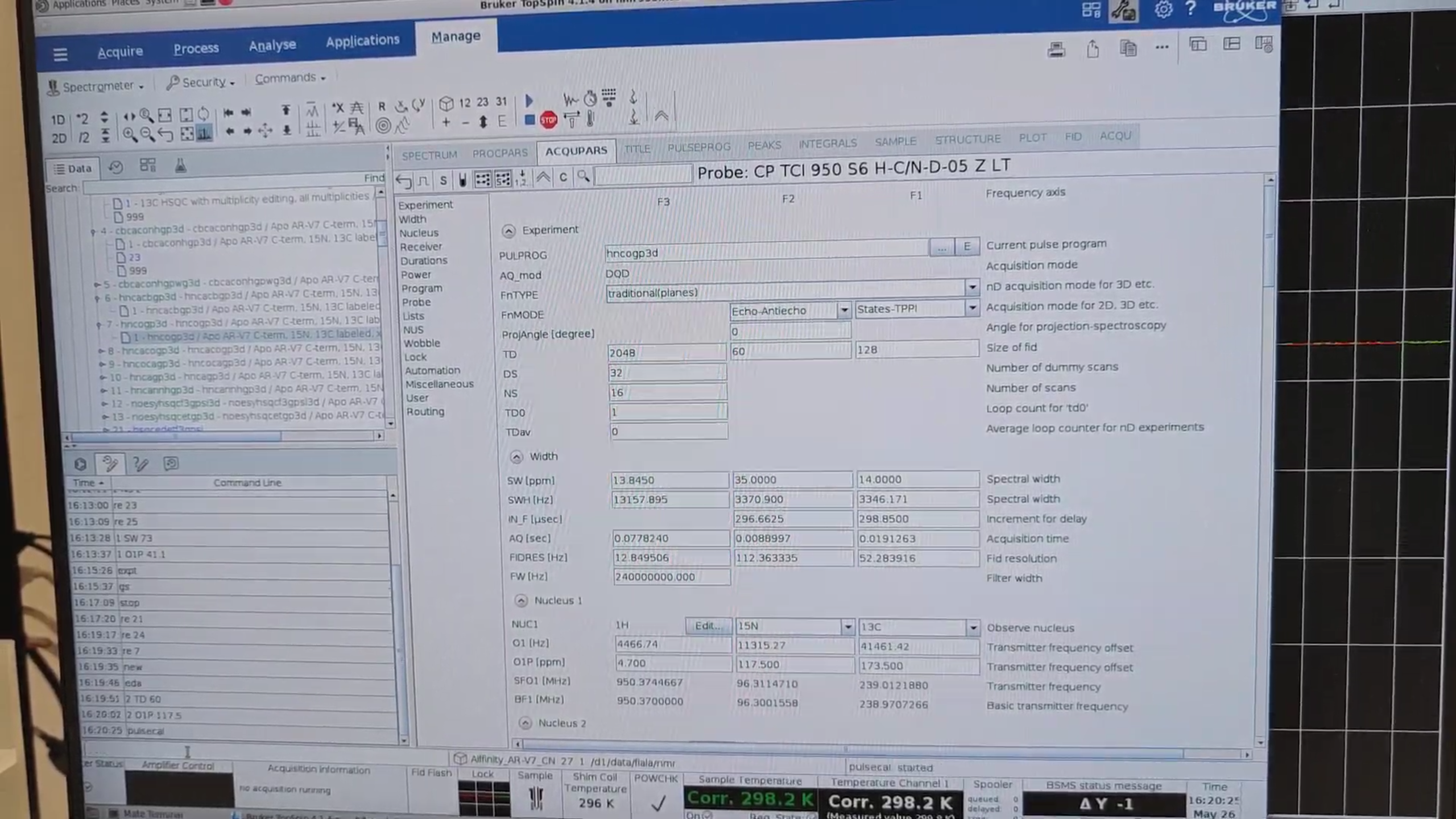
re 4 to load the selected standard CBCAcoNH, then new to create 23. In PROCPARS set:
| Parameter | Value |
|---|---|
TD{F2} |
60 |
TD{F1} |
128 |
SW{F1} |
73.0 ppm |
O1P{F1} |
41.1 ppm |
SW{F2} |
35 ppm (default value, keep it) |
O1P{F2} |
117.5 ppm |
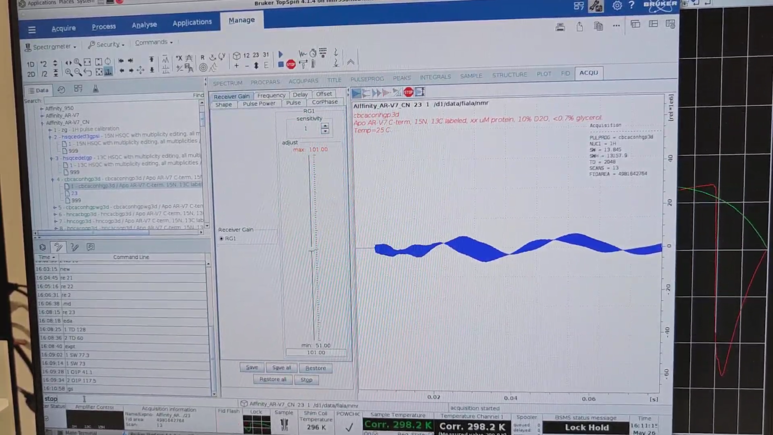
Because we have already measured the N–HN plane, we do not repeat pulsecal. Run gs (interactive acquisition) to
check that the experiment runs smoothly. TopSpin raises an error within seconds if, for example, a negative interval
occurs or the signal overflows. If everything is fine, press stop. Ideally, monitor the first increment only.
re 21, then new, to create a short QC 15N HSQC named 25 that checks protein stability. Adjust the Title, then eda and set:
| Parameter | Value |
|---|---|
NS |
2 |
5 · General 3D Motif
For each 3D experiment we will:
- Create the full-length 3D experiment.
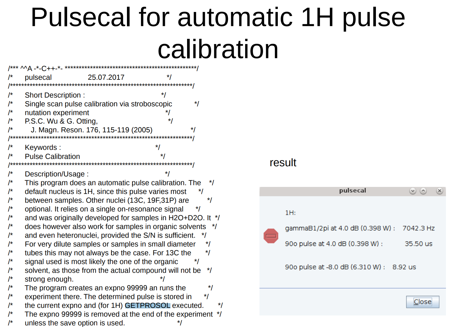
- Run
pulsecalto calibrate the 1H 90° pulse. A window shows the 90° pulse and its power level; click OK to accept. - Record a short QC 15N HSQC after the 3D experiment.
6 · HNCACB (exp. 25)
re 6, then new → 25. In eda set:
| Parameter | Value |
|---|---|
SW{F1} |
73.0 ppm |
O1P{F1} |
41.1 ppm |
O1P{F2} |
117.5 ppm |
Run pulsecal (automatic 1H 90° calibration). After collecting some data this command will pop up a window with a
90o pulse and its associated power level. Clicking “OK” will enter the displayed values into the current parameter set.
For 13C and 15N we used the default parameters in the “prosol” parameters table (command getprosol). If we wanted to
optimize the 13C 90o pulse and 15N 90o pulse, there are special calibration pulse sequences which we should have launched as
individual experiments (zg command).
Run gs; if no error appears, press stop.
Create QC 15N HSQC: re 24 → new → 26.
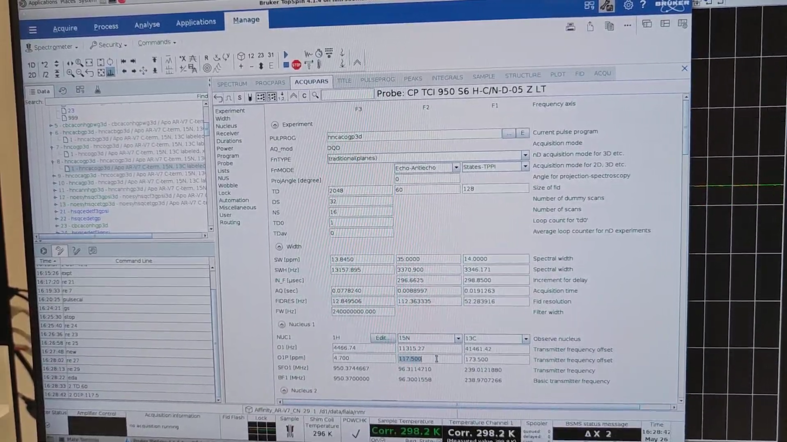
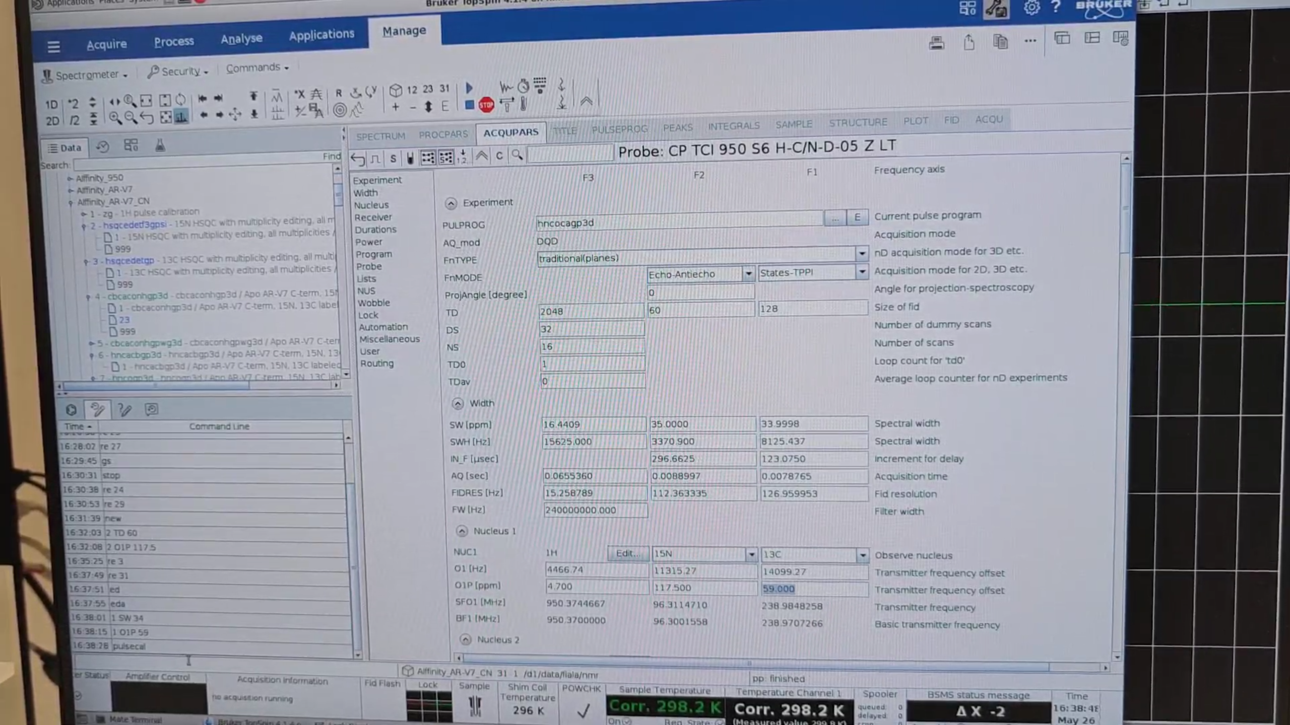
7 · HNCO (exp. 27)
re 7, new → 27. In eda set:
| Parameter | Value |
|---|---|
TD{F2} |
60 |
O1P{F2} |
117.5 ppm |
Run pulsecal, then gs, then stop.
Create QC 15N HSQC → re 24 → new → 28.
8 · HNcaCO (exp. 29)
re 8, new → 29. Set:
| Parameter | Value |
|---|---|
TD{F2} |
60 |
O1P{F2} |
117.5 ppm |
Run pulsecal, gs, stop.
Create QC 15N HSQC → re 24 → new → 30.
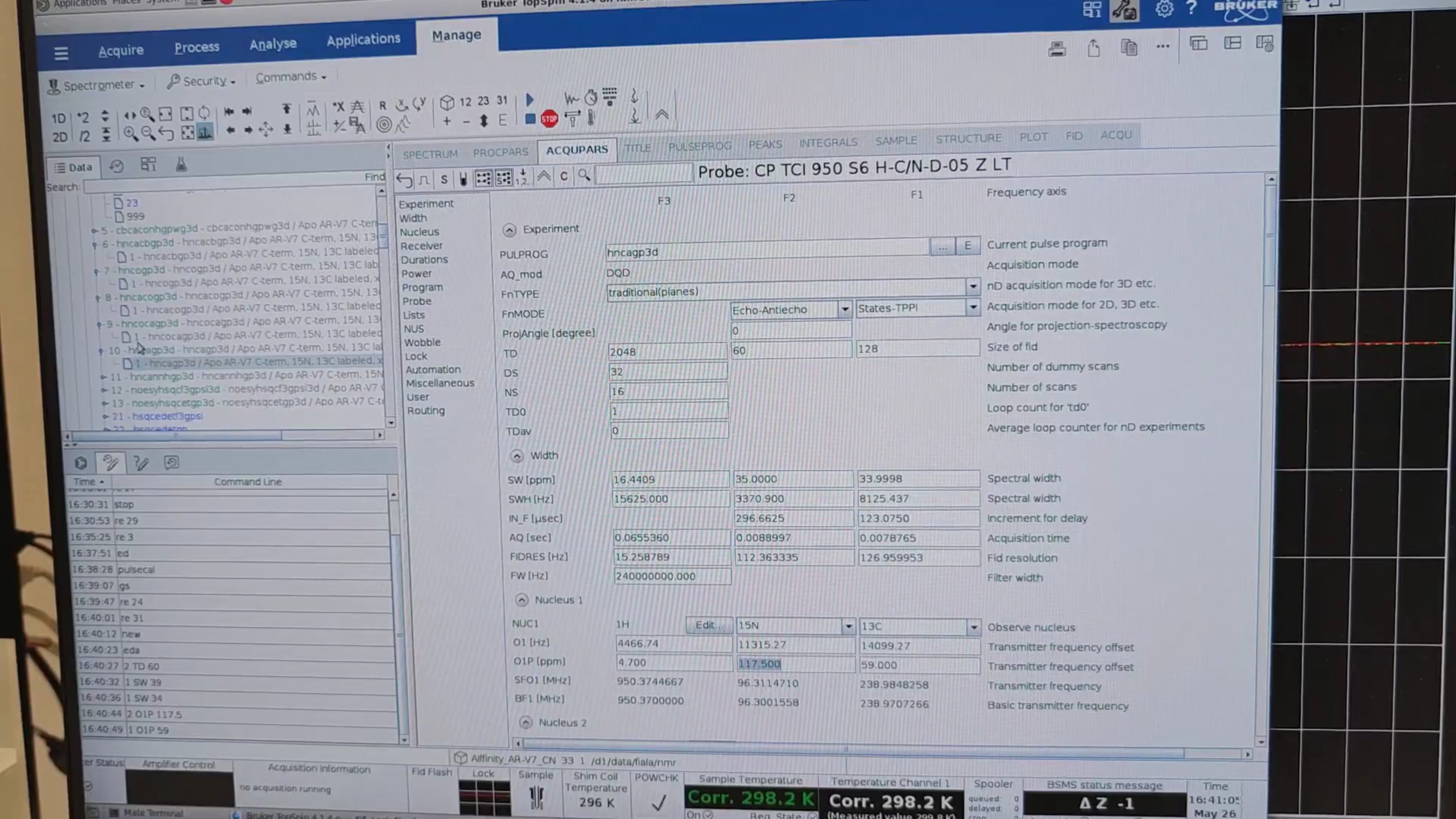
9 · HNcoCA (exp. 31)
re 3, zoom into the CA–HA region, and save the C range (e.g. 42–76 ppm).
re 9, new → 31. In eda set:
| Parameter | Value |
|---|---|
TD{F2} |
60 |
SW{F1} |
76−42 ppm |
O1P{F1} |
42+(76−42)/2 ppm |
O1P{F2} |
117.5 ppm |
Run pulsecal, gs, stop.
Create QC 15N HSQC → re 24 → new → 32.
10 · HNCA (exp. 33)
re 10, new → 33. Use the same CA window (42–76 ppm) and set:
| Parameter | Value |
|---|---|
TD{F2} |
60 |
SW{F1} |
76-42 ppm |
O1P{F1} |
42+(76-42)/2 ppm |
O1P{F2} |
117.5 ppm |
Run pulsecal, gs, stop.
Create QC 15N HSQC → re 24 → new → 34.
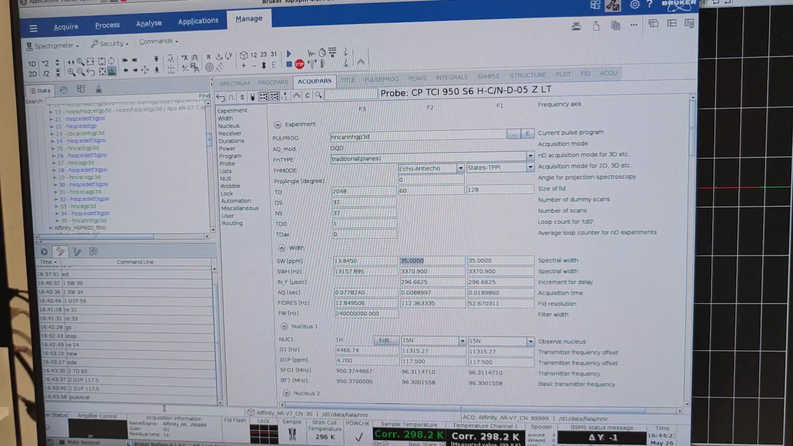
11 · hNcaNNH (exp. 35)
re 11, new → 35. Then set:
| Parameter | Value |
|---|---|
TD{F2} |
60 |
SW{F1} |
35 ppm (keep) |
SW{F2} |
35 ppm (keep) |
O1P{F1} |
117.5 ppm |
O1P{F2} |
117.5 ppm |
Run pulsecal, gs, stop.
Create QC 15N HSQC: re 24 → new → 36.
12 · Queue Management
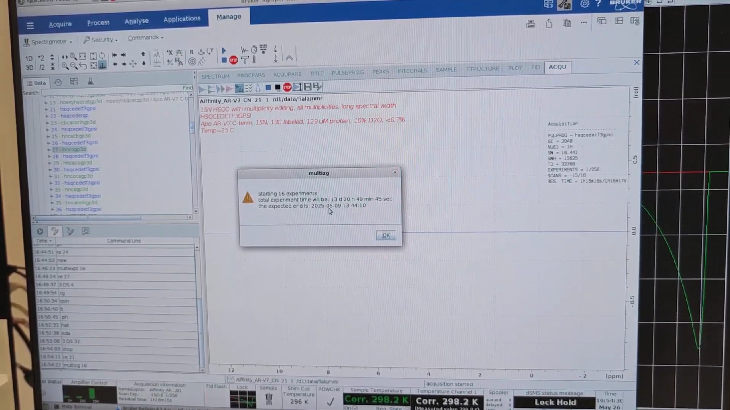
re 21, then multiexpt 16 to estimate the total time for all 16 experiments.
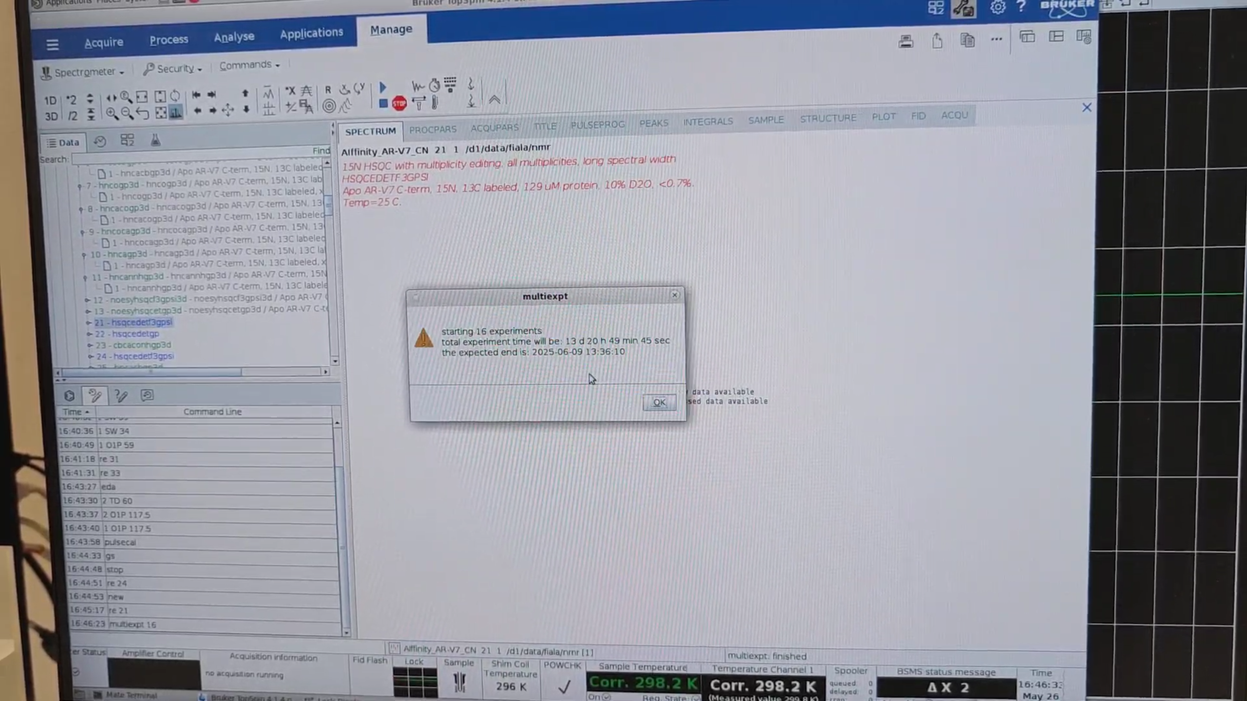
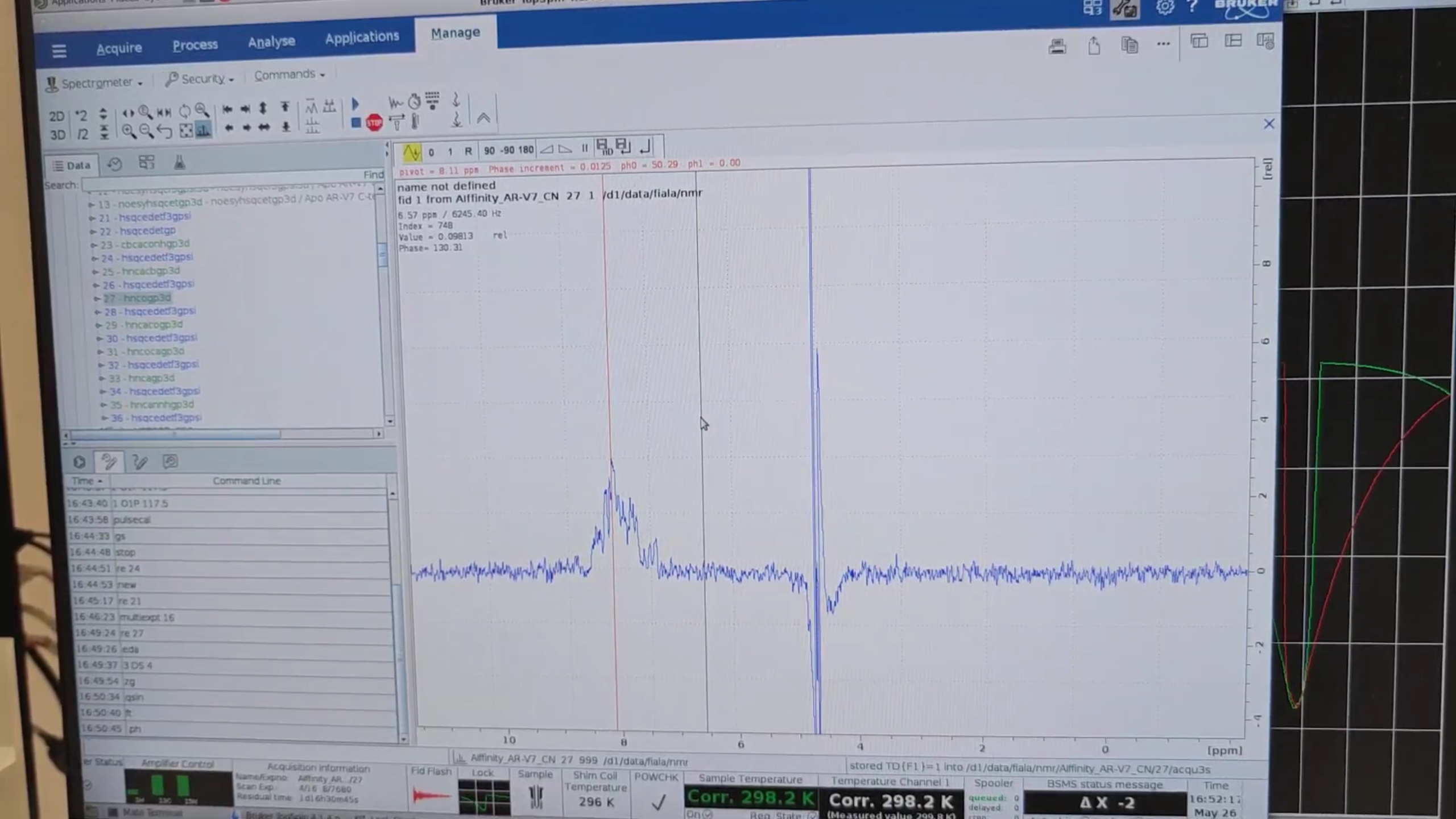
re 27 to switch to HNCO (the most sensitive 3D). In eda set DS = 4, then zg to acquire one increment. When
finished, run qsin, ft, .ph. After confirming protein signal, stop with halt (or stop) and reset DS back to 32.
Finally, re 21, then multizg 16 to launch all experiments serially.
Notes
- The 3D experiments employ shaped pulses, unlike the 2D HSQCs.
pulsecaloptimises the 1H 90° pulse and recalculates all shaped pulses (including decoupling) with the new value. Otherwise, we would have to copy the calibrated 1H 90° pulse parameters from the 2D to the 3D experiment and optimise each shaped pulse manually. - HSQC spectra define the H, C and N windows (
SW,O1P) that we copy into the 3D experiment setups. TD(size of FID),SW(spectral width) andAQ(acquisition time) are inter-dependent: setting any two automatically determines the third in TopSpin.
Authors
- Thomas Evangelidis